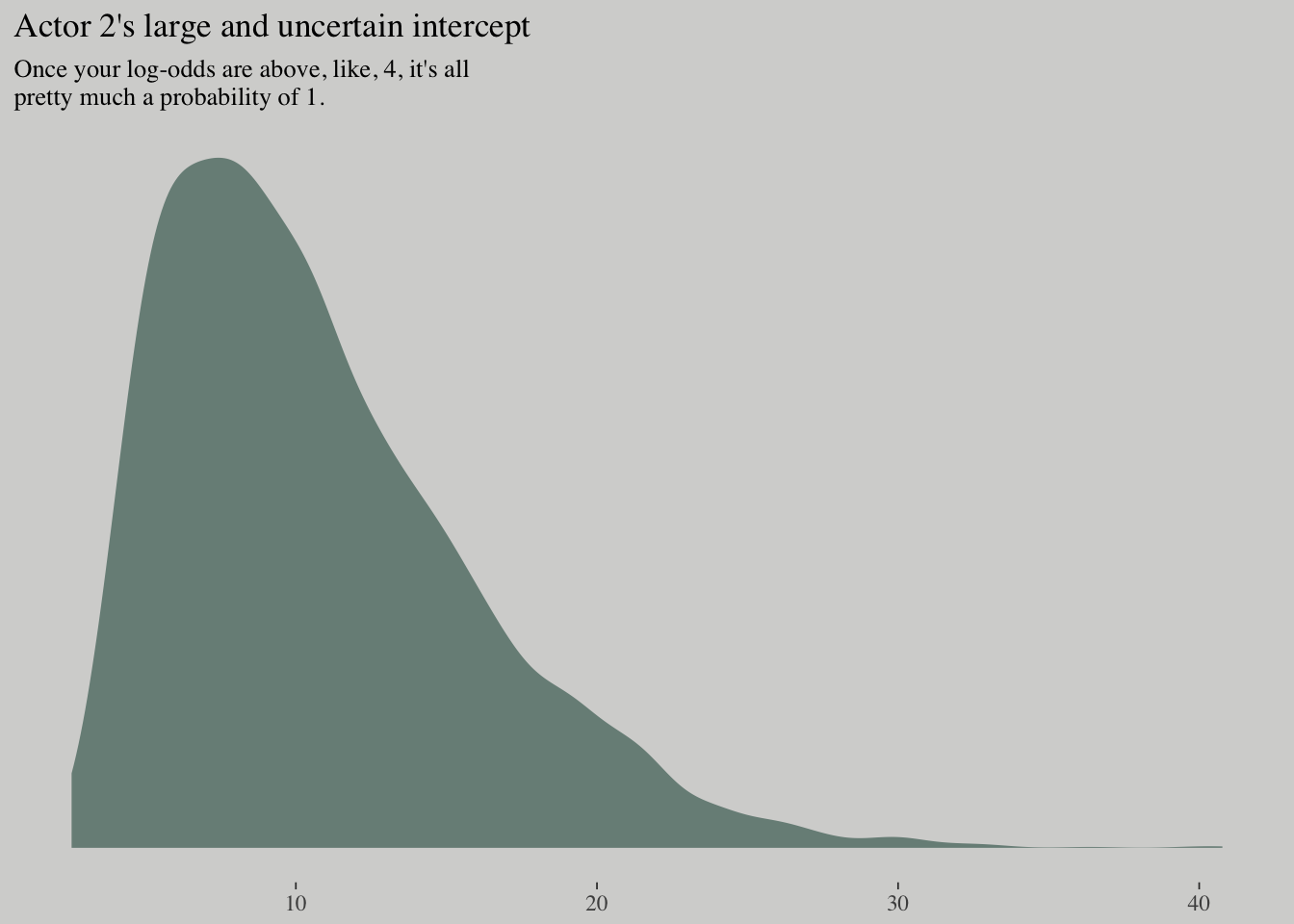
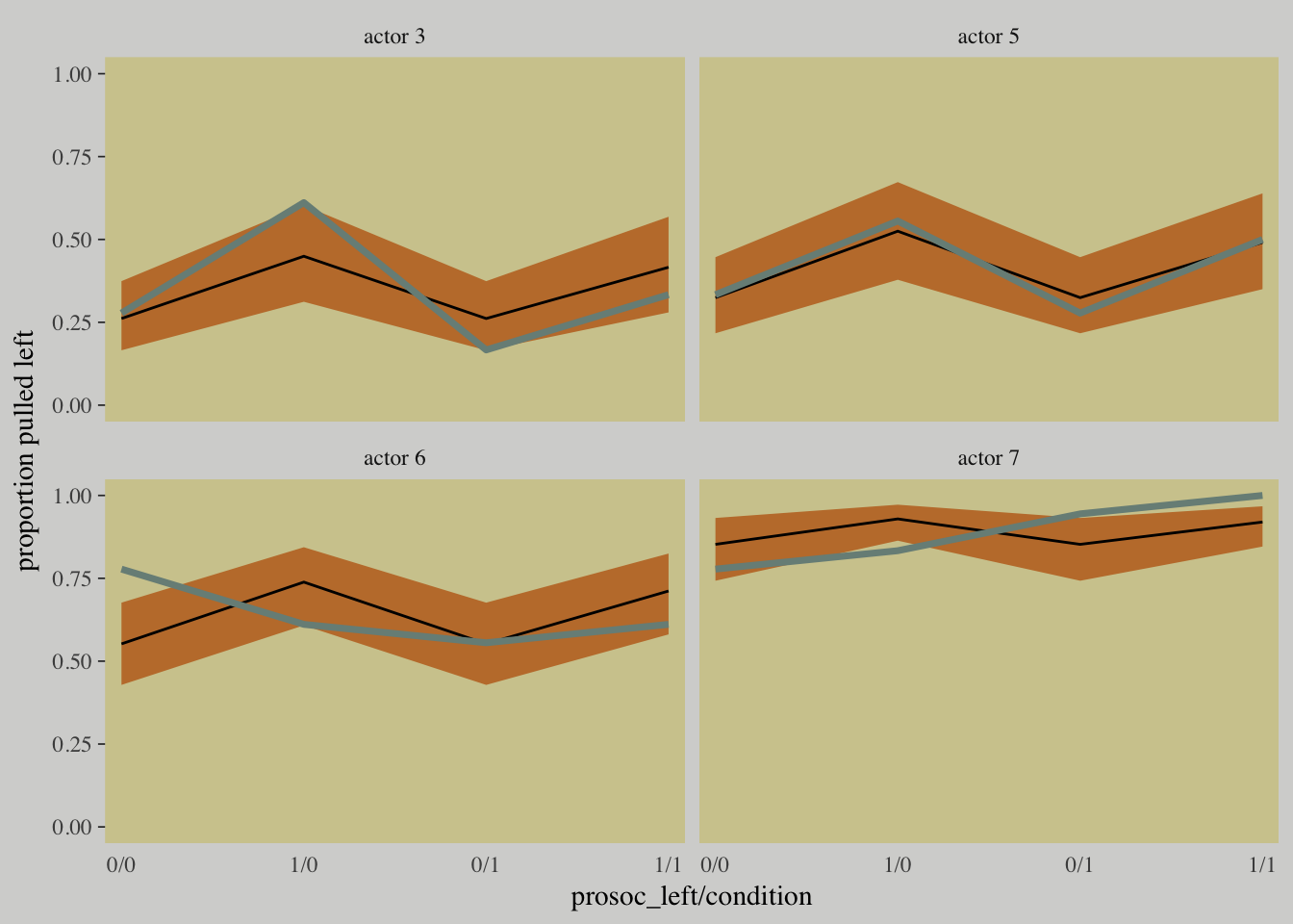
A fundamental difficulty with these models is that parameters are on a different scale, typically log-odds (for binomial) or log-rate (for Poisson), than the outcome variable they describe.
10.1. Binomial regression
A family of related procedures that model a binary classification for which the total of both categories is known.
The binomial distribution is denoted as:
\[y \sim \text{Binomial}\left( n,p \right) \]
where \(y\) is a count (zero or a positive whole number), \(p\) is the probability any particular “trial” is a success, and \(n\) is the number of trials.
As the basis for a generalized linear model, the binomial distribution has maximum entropy when each trial must result in one of two events and the expected value is constant.
There are two common flavors of GLM that use binomial likelihood functions:
- Logistic regression is the common name when the data are organized into single-trial cases, such that the outcome variable can only take values 0 and 1.
- When individual trials with the same covariate values are instead aggregated together, it is common to speak of an aggregated binomial regression. In this case, the outcome can take the value zero or any positive integer up to n, the number of trials.
It is important to never convert counts to proportions before analysis, because doing so destroys information about sample size.
10.1.2. Aggregated binomial: Chimpanzees again, condensed
d_aggregated <-
    d %>%
    select(-recipient, -block, -trial, -chose_prosoc) %>%
    group_by(actor, condition, prosoc_left) %>%
    summarise(x = sum(pulled_left))

d_aggregated %>%
    slice(1:8)
## # A tibble: 28 x 4
## # Groups: actor, condition [14]
## actor condition prosoc_left x
## <int> <int> <int> <int>
## 1 1 0 0 6
## 2 1 0 1 9
## 3 1 1 0 5
## 4 1 1 1 10
## 5 2 0 0 18
## 6 2 0 1 18
## 7 2 1 0 18
## 8 2 1 1 18
## 9 3 0 0 5
## 10 3 0 1 11
## # ... with 18 more rowsm10.5 <-
brm(data = d_aggregated, family = binomial,
x | trials(18) ~ 1 + prosoc_left + condition:prosoc_left ,
prior = c(set_prior("normal(0, 10)", class = "Intercept"),
set_prior("normal(0, 10)", class = "b")),
iter = 2500, warmup = 500, cores = 2, chains = 2)Comparing the models:
fixef(m10.3) %>% round(digits = 2)## Estimate Est.Error 2.5%ile 97.5%ile
## Intercept 0.05 0.13 -0.21 0.29
## prosoc_left 0.61 0.23 0.17 1.08
## prosoc_left:condition -0.11 0.27 -0.63 0.42fixef(m10.5) %>% round(digits = 2)## Estimate Est.Error 2.5%ile 97.5%ile
## Intercept 0.05 0.13 -0.21 0.29
## prosoc_left 0.61 0.23 0.16 1.06
## prosoc_left:condition -0.10 0.27 -0.63 0.4010.1.3. Aggregated binomial: Graduate school admissions
library(rethinking)## rethinking (Version 1.59)##
## Attaching package: 'rethinking'## The following object is masked from 'package:purrr':
##
## map## The following objects are masked from 'package:brms':
##
## LOO, stancode, WAICdata(UCBadmit)
d <- UCBadmit
detach(package:rethinking)
library(brms)
rm(UCBadmit)
d <-
d %>%
mutate(male = ifelse(applicant.gender == "male", 1, 0))
d## dept applicant.gender admit reject applications male
## 1 A male 512 313 825 1
## 2 A female 89 19 108 0
## 3 B male 353 207 560 1
## 4 B female 17 8 25 0
## 5 C male 120 205 325 1
## 6 C female 202 391 593 0
## 7 D male 138 279 417 1
## 8 D female 131 244 375 0
## 9 E male 53 138 191 1
## 10 E female 94 299 393 0
## 11 F male 22 351 373 1
## 12 F female 24 317 341 0m10.6 <- brm(admit | trials(applications) ~ 1 + male, data = d, family = binomial,
prior = c(set_prior("normal(0, 10)", class = "Intercept"),
set_prior("normal(0, 10)", class = "b")),
iter = 2500, warmup = 500, cores = 2, chains = 2)
m10.7 <- brm(admit | trials(applications) ~ 1, data = d, family = binomial,
prior = c(set_prior("normal(0, 10)", class = "Intercept")),
iter = 2500, warmup = 500, cores = 2, chains = 2)loo::compare(waic(m10.6), waic(m10.7))## elpd_diff se
## -27.3 82.3post <- posterior_samples(m10.6)
post %>%
mutate(p_admit_male = invlogit(b_Intercept + b_male),
p_admit_female = invlogit(b_Intercept),
diff_admit = p_admit_male - p_admit_female) %>%
summarise(`2.5%` = quantile(diff_admit, probs = .025),
`50%` = median(diff_admit),
`97.5%` = quantile(diff_admit, probs = .975))## 2.5% 50% 97.5%
## 1 0.1138293 0.1417092 0.1694741d <-
d %>%
mutate(case = factor(1:12))
p_10.6 <-
fitted(m10.6) %>%
as_tibble() %>%
bind_cols(d)
d_text <-
d %>%
group_by(dept) %>%
summarise(case = mean(as.numeric(case)),
admit = mean(admit/applications) + .05)
ggplot(data = d, aes(x = case, y = admit/applications)) +
geom_pointrange(data = p_10.6,
aes(y = Estimate/applications,
ymin = `2.5%ile`/applications ,
ymax = `97.5%ile`/applications),
color = wes_palette("Moonrise2")[1],
shape = 1, alpha = 1/3) +
geom_point(color = wes_palette("Moonrise2")[2]) +
geom_line(aes(group = dept),
color = wes_palette("Moonrise2")[2]) +
geom_text(data = d_text,
aes(y = admit, label = dept),
color = wes_palette("Moonrise2")[2],
family = "serif") +
coord_cartesian(ylim = 0:1) +
labs(y = "Proportion admitted",
title = "Posterior validation check") +
theme(axis.ticks.x = element_blank())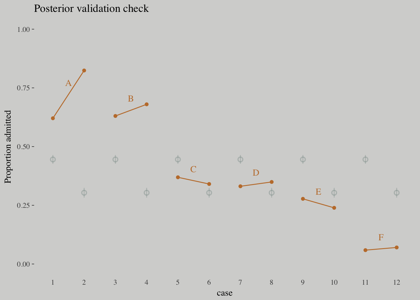
m10.8 <-
    brm(data = d, family = binomial,
        admit | trials(applications) ~ 0 + dept,
        prior = c(set_prior("normal(0, 10)", class = "b")),
        iter = 2500, warmup = 500, cores = 2, chains = 2)

m10.9 <-
    brm(data = d, family = binomial,
        admit | trials(applications) ~ 0 + dept + male ,
        prior = c(set_prior("normal(0, 10)", class = "b")),
        iter = 2500, warmup = 500, cores = 2, chains = 2)
fixef(m10.9) %>% round(digits = 2)## Estimate Est.Error 2.5%ile 97.5%ile
## deptA 0.68 0.10 0.48 0.88
## deptB 0.64 0.12 0.41 0.87
## deptC -0.58 0.08 -0.73 -0.44
## deptD -0.61 0.09 -0.79 -0.45
## deptE -1.06 0.10 -1.25 -0.87
## deptF -2.64 0.16 -2.95 -2.33
## male -0.10 0.08 -0.26 0.06m10.9$fit## Inference for Stan model: binomial brms-model.
## 2 chains, each with iter=2500; warmup=500; thin=1;
## post-warmup draws per chain=2000, total post-warmup draws=4000.
##
## mean se_mean sd 2.5% 25% 50% 75% 97.5% n_eff Rhat
## b_deptA 0.68 0.00 0.10 0.48 0.61 0.68 0.75 0.88 1955 1.00
## b_deptB 0.64 0.00 0.12 0.41 0.56 0.64 0.72 0.87 2098 1.00
## b_deptC -0.58 0.00 0.08 -0.73 -0.63 -0.58 -0.53 -0.44 4000 1.00
## b_deptD -0.61 0.00 0.09 -0.79 -0.67 -0.61 -0.56 -0.45 3132 1.00
## b_deptE -1.06 0.00 0.10 -1.25 -1.12 -1.06 -1.00 -0.87 4000 1.00
## b_deptF -2.64 0.00 0.16 -2.95 -2.74 -2.63 -2.53 -2.33 4000 1.00
## b_male -0.10 0.00 0.08 -0.26 -0.16 -0.10 -0.05 0.06 1600 1.01
## lp__ -70.67 0.05 1.88 -75.16 -71.75 -70.36 -69.26 -68.00 1636 1.00
##
## Samples were drawn using NUTS(diag_e) at Sat May 5 15:09:37 2018.
## For each parameter, n_eff is a crude measure of effective sample size,
## and Rhat is the potential scale reduction factor on split chains (at
## convergence, Rhat=1).loos <- loo(m10.6, m10.7, m10.8, m10.9,
reloo = T,
cores = 2)
loos## LOOIC SE
## m10.6 1026.58 337.43
## m10.7 1072.04 339.14
## m10.8 117.68 23.50
## m10.9 131.73 25.07
## m10.6 - m10.7 -45.46 165.98
## m10.6 - m10.8 908.90 331.46
## m10.6 - m10.9 894.84 333.19
## m10.7 - m10.8 954.36 330.87
## m10.7 - m10.9 940.31 331.23
## m10.8 - m10.9 -14.06 5.87d <-
d %>%
mutate(case = factor(1:12))
p_10.9 <-
fitted(m10.9) %>%
as_tibble() %>%
bind_cols(d)
d_text <-
d %>%
group_by(dept) %>%
summarise(case = mean(as.numeric(case)),
admit = mean(admit/applications) + .05)
ggplot(data = d, aes(x = case, y = admit/applications)) +
geom_pointrange(data = p_10.9,
aes(y = Estimate/applications,
ymin = `2.5%ile`/applications ,
ymax = `97.5%ile`/applications),
color = wes_palette("Moonrise2")[1],
shape = 1, alpha = 1/3) +
geom_point(color = wes_palette("Moonrise2")[2]) +
geom_line(aes(group = dept),
color = wes_palette("Moonrise2")[2]) +
geom_text(data = d_text,
aes(y = admit, label = dept),
color = wes_palette("Moonrise2")[2],
family = "serif") +
coord_cartesian(ylim = 0:1) +
labs(y = "Proportion admitted",
title = "Posterior validation check") +
theme(axis.ticks.x = element_blank())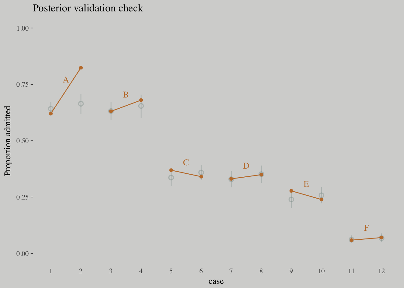
Information criteria digression
l_m10.6 <- LOO(m10.6)## Warning: Found 6 observations with a pareto_k > 0.7 in model 'm10.6'. It
## is recommended to set 'reloo = TRUE' in order to calculate the ELPD without
## the assumption that these observations are negligible. This will refit
## the model 6 times to compute the ELPDs for the problematic observations
## directly.l_m10.6##
## Computed from 4000 by 12 log-likelihood matrix
##
## Estimate SE
## elpd_loo -483.2 158.3
## p_loo 101.2 35.0
## looic 966.4 316.6
## ------
## Monte Carlo SE of elpd_loo is NA.
##
## Pareto k diagnostic values:
## Count Pct. Min. n_eff
## (-Inf, 0.5] (good) 4 33.3% 574
## (0.5, 0.7] (ok) 2 16.7% 378
## (0.7, 1] (bad) 2 16.7% 43
## (1, Inf) (very bad) 4 33.3% 1
## See help('pareto-k-diagnostic') for details.The Pareto \(k\) parameter can be used as a diagnostic tool. Each case in the data gets its own \(k\) value and we like it when those \(k\)s are low. The makers of the loo package get worried when those \(k\)s exceed 0.7 and as a result, loo() spits out a warning message when they do.
library(loo)
pareto_k_table(l_m10.6)
## Pareto k diagnostic values:
## Count Pct. Min. n_eff
## (-Inf, 0.5] (good) 4 33.3% 574
## (0.5, 0.7] (ok) 2 16.7% 378
## (0.7, 1] (bad) 2 16.7% 43
## (1, Inf) (very bad) 4 33.3% 1plot(l_m10.6)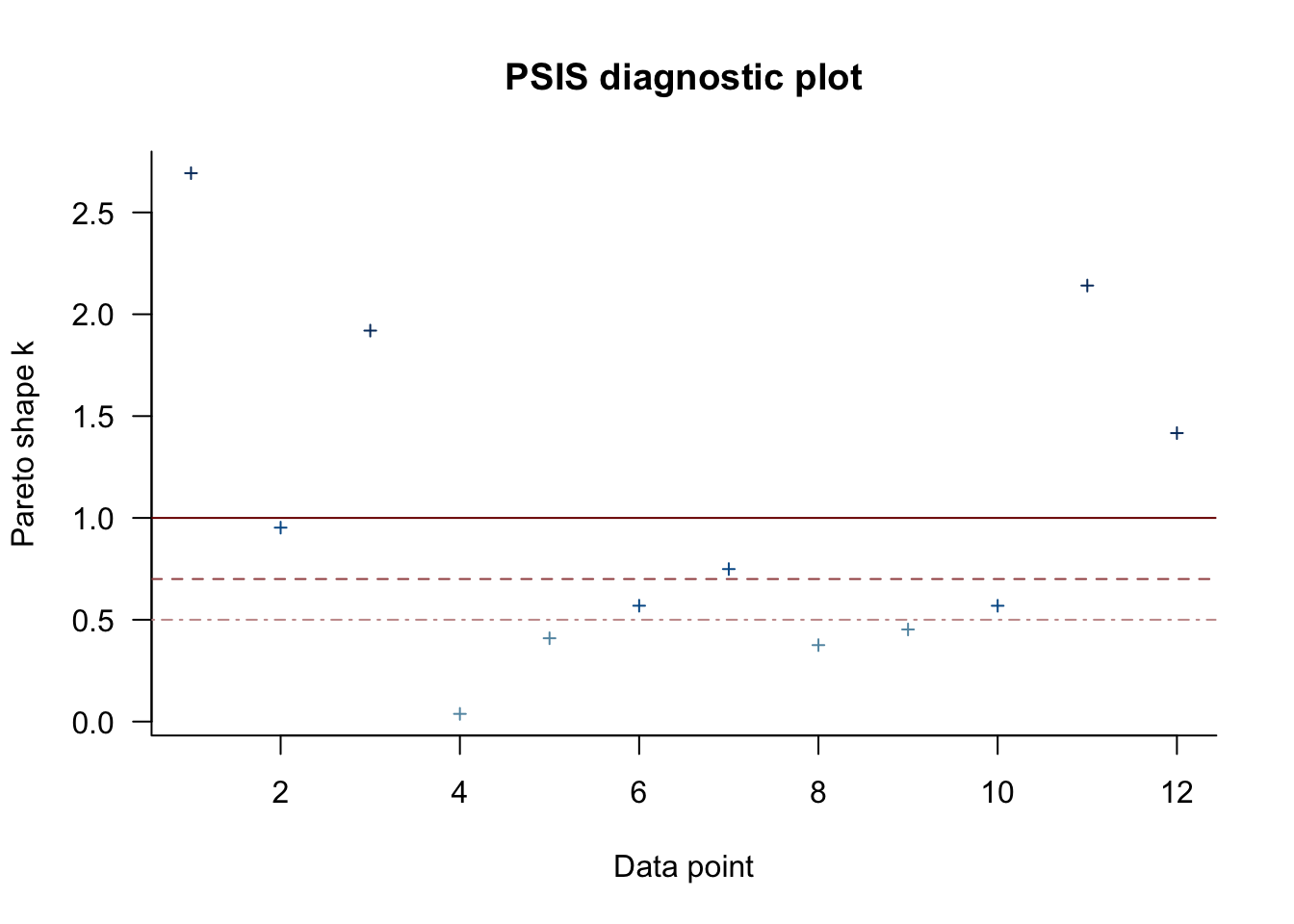
pareto_k_ids(l_m10.6, threshold = 1)## [1] 1 3 11 12l_m10.6_reloo <- LOO(m10.6, reloo = T)##
## Gradient evaluation took 3.4e-05 seconds
## 1000 transitions using 10 leapfrog steps per transition would take 0.34 seconds.
## Adjust your expectations accordingly!
##
##
##
## Elapsed Time: 0.054515 seconds (Warm-up)
## 0.077842 seconds (Sampling)
## 0.132357 seconds (Total)
##
##
## Gradient evaluation took 1.3e-05 seconds
## 1000 transitions using 10 leapfrog steps per transition would take 0.13 seconds.
## Adjust your expectations accordingly!
##
##
##
## Elapsed Time: 0.053537 seconds (Warm-up)
## 0.071429 seconds (Sampling)
## 0.124966 seconds (Total)
##
##
## Gradient evaluation took 1.5e-05 seconds
## 1000 transitions using 10 leapfrog steps per transition would take 0.15 seconds.
## Adjust your expectations accordingly!
##
##
##
## Elapsed Time: 0.054269 seconds (Warm-up)
## 0.063526 seconds (Sampling)
## 0.117795 seconds (Total)
##
##
## Gradient evaluation took 1.2e-05 seconds
## 1000 transitions using 10 leapfrog steps per transition would take 0.12 seconds.
## Adjust your expectations accordingly!
##
##
##
## Elapsed Time: 0.055782 seconds (Warm-up)
## 0.050451 seconds (Sampling)
## 0.106233 seconds (Total)
##
##
## Gradient evaluation took 1.5e-05 seconds
## 1000 transitions using 10 leapfrog steps per transition would take 0.15 seconds.
## Adjust your expectations accordingly!
##
##
##
## Elapsed Time: 0.057025 seconds (Warm-up)
## 0.06301 seconds (Sampling)
## 0.120035 seconds (Total)
##
##
## Gradient evaluation took 1.3e-05 seconds
## 1000 transitions using 10 leapfrog steps per transition would take 0.13 seconds.
## Adjust your expectations accordingly!
##
##
##
## Elapsed Time: 0.054462 seconds (Warm-up)
## 0.063167 seconds (Sampling)
## 0.117629 seconds (Total)
##
##
## Gradient evaluation took 1.6e-05 seconds
## 1000 transitions using 10 leapfrog steps per transition would take 0.16 seconds.
## Adjust your expectations accordingly!
##
##
##
## Elapsed Time: 0.055842 seconds (Warm-up)
## 0.058894 seconds (Sampling)
## 0.114736 seconds (Total)
##
##
## Gradient evaluation took 1.3e-05 seconds
## 1000 transitions using 10 leapfrog steps per transition would take 0.13 seconds.
## Adjust your expectations accordingly!
##
##
##
## Elapsed Time: 0.056581 seconds (Warm-up)
## 0.05565 seconds (Sampling)
## 0.112231 seconds (Total)
##
##
## Gradient evaluation took 1.5e-05 seconds
## 1000 transitions using 10 leapfrog steps per transition would take 0.15 seconds.
## Adjust your expectations accordingly!
##
##
##
## Elapsed Time: 0.056436 seconds (Warm-up)
## 0.061603 seconds (Sampling)
## 0.118039 seconds (Total)
##
##
## Gradient evaluation took 1.3e-05 seconds
## 1000 transitions using 10 leapfrog steps per transition would take 0.13 seconds.
## Adjust your expectations accordingly!
##
##
##
## Elapsed Time: 0.055733 seconds (Warm-up)
## 0.062833 seconds (Sampling)
## 0.118566 seconds (Total)
##
##
## Gradient evaluation took 1.5e-05 seconds
## 1000 transitions using 10 leapfrog steps per transition would take 0.15 seconds.
## Adjust your expectations accordingly!
##
##
##
## Elapsed Time: 0.054649 seconds (Warm-up)
## 0.054116 seconds (Sampling)
## 0.108765 seconds (Total)
##
##
## Gradient evaluation took 1.2e-05 seconds
## 1000 transitions using 10 leapfrog steps per transition would take 0.12 seconds.
## Adjust your expectations accordingly!
##
##
##
## Elapsed Time: 0.054765 seconds (Warm-up)
## 0.063091 seconds (Sampling)
## 0.117856 seconds (Total)l_m10.6_reloo##
## Computed from 4000 by 12 log-likelihood matrix
##
## Estimate SE
## elpd_loo -516.1 171.4
## p_loo 134.1 51.8
## looic 1032.3 342.9
## ------
## Monte Carlo SE of elpd_loo is NA.
##
## Pareto k diagnostic values:
## Count Pct. Min. n_eff
## (-Inf, 0.5] (good) 10 83.3% 1
## (0.5, 0.7] (ok) 2 16.7% 378
## (0.7, 1] (bad) 0 0.0% <NA>
## (1, Inf) (very bad) 0 0.0% <NA>
##
## All Pareto k estimates are ok (k < 0.7).
## See help('pareto-k-diagnostic') for details.Check this vignette on how the loo package’s Pareto (k) can help detect outliers.
10.1.4. Fitting binomial regressions with glm
# outcome and predictor almost perfectly associated
y <- c(rep(0, 10), rep(1, 10))
x <- c(rep(-1, 9), rep(1, 11))

b.good <-
    brm(data = list(y = y, x = x), family = bernoulli,
        y ~ 1 + x,
        prior = c(set_prior("normal(0, 10)", class = "Intercept"),
                  set_prior("normal(0, 10)", class = "b")))
##
## SAMPLING FOR MODEL 'bernoulli brms-model' NOW (CHAIN 1).
##
## Gradient evaluation took 3.1e-05 seconds
## 1000 transitions using 10 leapfrog steps per transition would take 0.31 seconds.
## Adjust your expectations accordingly!
##
##
## Iteration: 1 / 2000 [ 0%] (Warmup)
## Iteration: 200 / 2000 [ 10%] (Warmup)
## Iteration: 400 / 2000 [ 20%] (Warmup)
## Iteration: 600 / 2000 [ 30%] (Warmup)
## Iteration: 800 / 2000 [ 40%] (Warmup)
## Iteration: 1000 / 2000 [ 50%] (Warmup)
## Iteration: 1001 / 2000 [ 50%] (Sampling)
## Iteration: 1200 / 2000 [ 60%] (Sampling)
## Iteration: 1400 / 2000 [ 70%] (Sampling)
## Iteration: 1600 / 2000 [ 80%] (Sampling)
## Iteration: 1800 / 2000 [ 90%] (Sampling)
## Iteration: 2000 / 2000 [100%] (Sampling)
##
## Elapsed Time: 0.058758 seconds (Warm-up)
## 0.061854 seconds (Sampling)
## 0.120612 seconds (Total)
##
##
## SAMPLING FOR MODEL 'bernoulli brms-model' NOW (CHAIN 2).
##
## Gradient evaluation took 8e-06 seconds
## 1000 transitions using 10 leapfrog steps per transition would take 0.08 seconds.
## Adjust your expectations accordingly!
##
##
## Iteration: 1 / 2000 [ 0%] (Warmup)
## Iteration: 200 / 2000 [ 10%] (Warmup)
## Iteration: 400 / 2000 [ 20%] (Warmup)
## Iteration: 600 / 2000 [ 30%] (Warmup)
## Iteration: 800 / 2000 [ 40%] (Warmup)
## Iteration: 1000 / 2000 [ 50%] (Warmup)
## Iteration: 1001 / 2000 [ 50%] (Sampling)
## Iteration: 1200 / 2000 [ 60%] (Sampling)
## Iteration: 1400 / 2000 [ 70%] (Sampling)
## Iteration: 1600 / 2000 [ 80%] (Sampling)
## Iteration: 1800 / 2000 [ 90%] (Sampling)
## Iteration: 2000 / 2000 [100%] (Sampling)
##
## Elapsed Time: 0.056059 seconds (Warm-up)
## 0.060835 seconds (Sampling)
## 0.116894 seconds (Total)
##
##
## SAMPLING FOR MODEL 'bernoulli brms-model' NOW (CHAIN 3).
##
## Gradient evaluation took 9e-06 seconds
## 1000 transitions using 10 leapfrog steps per transition would take 0.09 seconds.
## Adjust your expectations accordingly!
##
##
## Iteration: 1 / 2000 [ 0%] (Warmup)
## Iteration: 200 / 2000 [ 10%] (Warmup)
## Iteration: 400 / 2000 [ 20%] (Warmup)
## Iteration: 600 / 2000 [ 30%] (Warmup)
## Iteration: 800 / 2000 [ 40%] (Warmup)
## Iteration: 1000 / 2000 [ 50%] (Warmup)
## Iteration: 1001 / 2000 [ 50%] (Sampling)
## Iteration: 1200 / 2000 [ 60%] (Sampling)
## Iteration: 1400 / 2000 [ 70%] (Sampling)
## Iteration: 1600 / 2000 [ 80%] (Sampling)
## Iteration: 1800 / 2000 [ 90%] (Sampling)
## Iteration: 2000 / 2000 [100%] (Sampling)
##
## Elapsed Time: 0.055012 seconds (Warm-up)
## 0.04879 seconds (Sampling)
## 0.103802 seconds (Total)
##
##
## SAMPLING FOR MODEL 'bernoulli brms-model' NOW (CHAIN 4).
##
## Gradient evaluation took 9e-06 seconds
## 1000 transitions using 10 leapfrog steps per transition would take 0.09 seconds.
## Adjust your expectations accordingly!
##
##
## Iteration: 1 / 2000 [ 0%] (Warmup)
## Iteration: 200 / 2000 [ 10%] (Warmup)
## Iteration: 400 / 2000 [ 20%] (Warmup)
## Iteration: 600 / 2000 [ 30%] (Warmup)
## Iteration: 800 / 2000 [ 40%] (Warmup)
## Iteration: 1000 / 2000 [ 50%] (Warmup)
## Iteration: 1001 / 2000 [ 50%] (Sampling)
## Iteration: 1200 / 2000 [ 60%] (Sampling)
## Iteration: 1400 / 2000 [ 70%] (Sampling)
## Iteration: 1600 / 2000 [ 80%] (Sampling)
## Iteration: 1800 / 2000 [ 90%] (Sampling)
## Iteration: 2000 / 2000 [100%] (Sampling)
##
## Elapsed Time: 0.058365 seconds (Warm-up)
## 0.055513 seconds (Sampling)
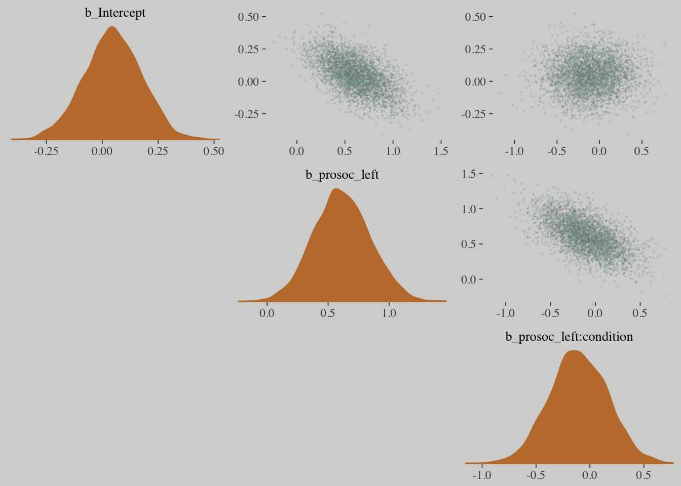
## 0.113878 seconds (Total)pairs(b.good,
off_diag_args = list(size = 1/10, alpha = 1/6))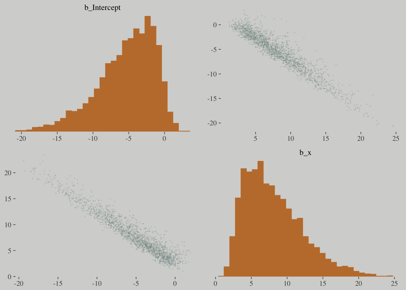
10.2. Poisson regression
It is a GLM that models a count outcome without a known maximum. The Poisson model can also be conceived of as a binomial model with a very large maximum but a very small probability per trial.
A Poisson distribution is useful because it allows us to model binomial events for which the number of trials \(n\) is unknown or uncountably large.
\[y \sim \text{Poisson} \left( \lambda \right)\]
where \(\lambda\) is the expected value of the outcome \(y\).
To build a GLM with this likelihood, the conventional link function for a Poisson model is the log link, i.e.
\[\begin{eqnarray} { y }_{ i } & \sim & \text{Poisson}\left( \lambda_i \right) \\ \log \left( { \lambda }_{ i } \right) & = & \alpha + \beta x_i \end{eqnarray}\]
Exponential relationships grow very quickly, and few natural phenomena can remain exponential for long. So one thing to always check with a log link is whether it makes sense at all ranges of the predictor variables.
The parameter \(\lambda\) is the expected value, but it’s also commonly thought of as a rate. Both interpretations are correct, and realizing this allows us to make Poisson models for which the exposure varies across cases \(i\).
Implicitly, \(\lambda\) is equal to an expected number of events, \(\mu\), per unit time or distance, \(\tau\). This implies that \(\lambda = \mu / \tau\), which lets us redefine the link:
\[\begin{eqnarray} { y }_{ i } & \sim & \text{Poisson}\left( \lambda_i \right) \\ \log { \lambda }_{ i } & = & \log { \frac { { \mu }_{ i } }{ { \tau }_{ i } } } =\log { { \mu }_{ i } } -\log { { \tau }_{ i } } = \alpha + \beta x_i \end{eqnarray}\]
The \(\tau\) values are the exposures. When the exposure varies across cases, then \(\tau_i\) does the important work of correctly scaling the expected number of events for each case \(i\). So you can model cases with different exposures just by adding a predictor, the logarithm of the exposure, without adding a parameter for it.
\[\begin{eqnarray} { y }_{ i } & \sim & \text{Poisson}\left( \mu_i \right) \\ \log { \mu }_{ i } & = & \log { { \tau }_{ i } } + \alpha + \beta x_i \end{eqnarray}\]
10.2.1. Example: Oceanic tool complexity
library(rethinking)
data(Kline)
d <- Kline
detach(package:rethinking)
library(brms)
rm(Kline)

d <-
  d %>%
  mutate(log_pop = log(population),
         contact_high = ifelse(contact == "high", 1, 0))

d
## culture population contact total_tools mean_TU log_pop
## 1 Malekula 1100 low 13 3.2 7.003065
## 2 Tikopia 1500 low 22 4.7 7.313220
## 3 Santa Cruz 3600 low 24 4.0 8.188689
## 4 Yap 4791 high 43 5.0 8.474494
## 5 Lau Fiji 7400 high 33 5.0 8.909235
## 6 Trobriand 8000 high 19 4.0 8.987197
## 7 Chuuk 9200 high 40 3.8 9.126959
## 8 Manus 13000 low 28 6.6 9.472705
## 9 Tonga 17500 high 55 5.4 9.769956
## 10 Hawaii 275000 low 71 6.6 12.524526
## contact_high
## 1 0
## 2 0
## 3 0
## 4 1
## 5 1
## 6 1
## 7 1
## 8 0
## 9 1
## 10 0The model to consider is:
\[\begin{eqnarray} { T }_{ i } & \sim & \text{Poisson}\left( \lambda_i \right) \\ \log \left( { \lambda }_{ i } \right) & = & \alpha + { \beta }_{ P } \log P_i + { \beta }_{ C } C_i + { \beta }_{ PC } C_i \log P_i \\ \alpha & \sim & \text{Normal}(0,100) \\ { \beta }_{ P } & \sim & \text{Normal}(0,1) \\ { \beta }_{ C } & \sim & \text{Normal}(0,1) \\ { \beta }_{ PC } & \sim & \text{Normal}(0,1) \end{eqnarray}\]
Strongly regularizing priors are used because the sample is small, so we should fear overfitting more. And since the predictors are not centered, there’s no telling where \(\alpha\) should end up, so an essentially flat prior is assigned to it.
m10.10 <- brm(data = d, family = poisson,
              total_tools ~ 1 + log_pop + contact_high + contact_high:log_pop,
              prior = c(set_prior("normal(0, 100)", class = "Intercept"),
                        set_prior("normal(0, 1)", class = "b")),
              iter = 3000, warmup = 1000, chains = 4, cores = 4)

print(m10.10)
## Family: poisson
## Links: mu = log
## Formula: total_tools ~ 1 + log_pop + contact_high + contact_high:log_pop
## Data: d (Number of observations: 10)
## Samples: 4 chains, each with iter = 3000; warmup = 1000; thin = 1;
## total post-warmup samples = 8000
## ICs: LOO = NA; WAIC = NA; R2 = NA
##
## Population-Level Effects:
## Estimate Est.Error l-95% CI u-95% CI Eff.Sample Rhat
## Intercept 0.94 0.36 0.21 1.62 4036 1.00
## log_pop 0.26 0.04 0.20 0.33 4253 1.00
## contact_high -0.10 0.84 -1.75 1.55 3277 1.00
## log_pop:contact_high 0.04 0.09 -0.14 0.22 3303 1.00
##
## Samples were drawn using sampling(NUTS). For each parameter, Eff.Sample
## is a crude measure of effective sample size, and Rhat is the potential
## scale reduction factor on split chains (at convergence, Rhat = 1).post <-
posterior_samples(m10.10)
post %>%
select(-lp__) %>%
rename(b_interaction = `b_log_pop:contact_high`) %>%
cor() %>%
round(digits = 2)## b_Intercept b_log_pop b_contact_high b_interaction
## b_Intercept 1.00 -0.98 -0.12 0.06
## b_log_pop -0.98 1.00 0.12 -0.08
## b_contact_high -0.12 0.12 1.00 -0.99
## b_interaction 0.06 -0.08 -0.99 1.00# We'll set a renewed color theme
color_scheme_set(c(wes_palette("Moonrise2")[2],
wes_palette("Moonrise2")[1],
wes_palette("Moonrise2")[4],
wes_palette("Moonrise2")[2],
wes_palette("Moonrise2")[1],
wes_palette("Moonrise2")[1]))
post %>%
select(-lp__) %>%
rename(b_interaction = `b_log_pop:contact_high`) %>%
mcmc_intervals(prob = .5, prob_outer = .95) +
theme(axis.ticks.y = element_blank(),
axis.text.y = element_text(hjust = 0))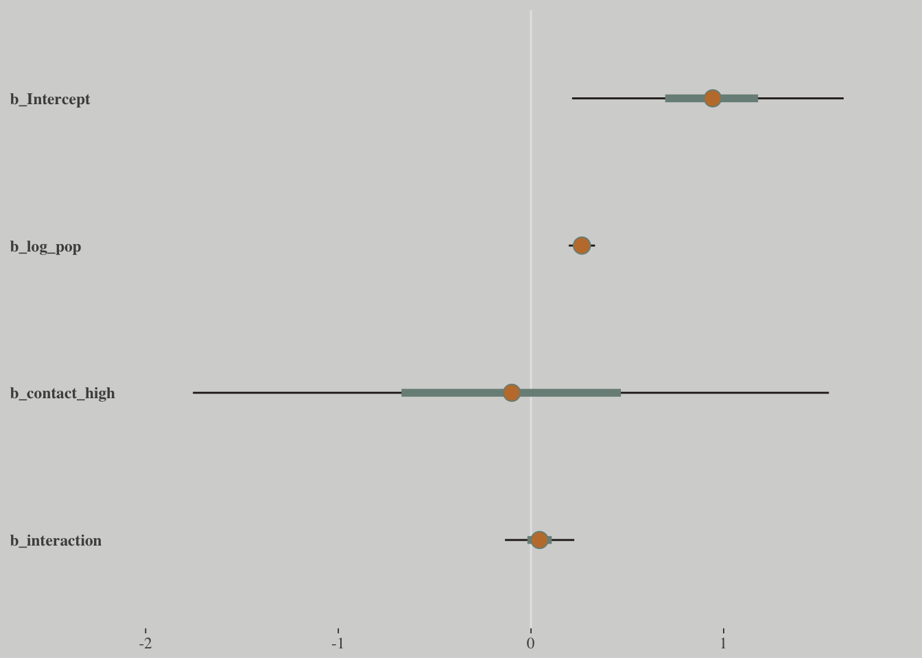
Check if contact rate has no impact on prediction in this model:
post <-
    post %>%
    mutate(lambda_high = exp(b_Intercept + b_contact_high + (b_log_pop + `b_log_pop:contact_high`)*8),
           lambda_low = exp(b_Intercept + b_log_pop*8),
           diff = lambda_high - lambda_low)

post %>%
    summarise(sum = sum(diff > 0)/length(diff))
## sum
## 1 0.959625post %>%
ggplot(aes(x = diff)) +
geom_density(color = "transparent",
fill = wes_palette("Moonrise2")[1]) +
geom_vline(xintercept = 0, linetype = 2,
color = wes_palette("Moonrise2")[2]) +
scale_y_continuous(NULL, breaks = NULL) +
labs(x = "lambda_high - lambda_low")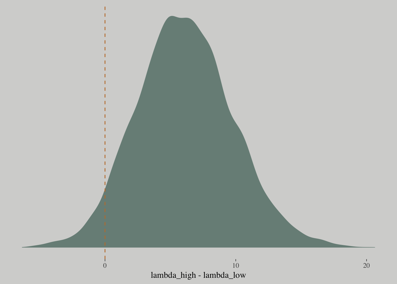
# Intermediary tibbles for our the dot and line portoin of the plot
point_tibble <-
    tibble(x = c(median(post$b_contact_high), min(post$b_contact_high)),
           y = c(min(post$`b_log_pop:contact_high`), median(post$`b_log_pop:contact_high`)))

line_tibble <-
    tibble(parameter = rep(c("b_contact_high", "b_log_pop:contact_high"), each = 2),
           x = c(quantile(post$b_contact_high, probs = c(.025, .975)),
                 rep(min(post$b_contact_high), times = 2)),
           y = c(rep(min(post$`b_log_pop:contact_high`), times = 2),
                 quantile(post$`b_log_pop:contact_high`, probs = c(.025, .975))))

# the plot
post %>%
    ggplot(aes(x = b_contact_high, y = `b_log_pop:contact_high`)) +
    geom_point(color = wes_palette("Moonrise2")[1],
               size = 1/10, alpha = 1/10) +
    geom_point(data = point_tibble,
               aes(x = x, y = y)) +
    geom_line(data = line_tibble,
              aes(x = x, y = y, group = parameter)) +
    labs(subtitle = "Neither parameter is conventionally “significant,” but together they imply\nthat contact rate consistently influences prediction.")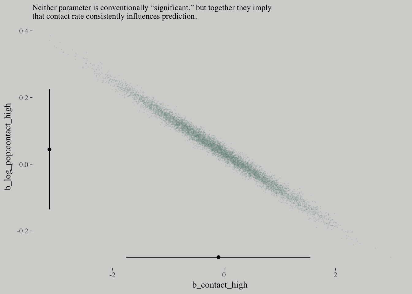
How can contact rate be significant when both
b_contact_highandb_interactionare, conventionally speaking, non-significant? One reason is because the uncertainty in the parameters is correlated.
You can’t just inspect the marginal uncertainty in each parameter from the table of estimates, and get an accurate understanding of the impact of the joint uncertainty on prediction.
# no interaction
m10.11 <-
    update(m10.10, formula = total_tools ~ 1 + log_pop + contact_high,
           iter = 3000, warmup = 1000, chains = 4, cores = 4)

# no contact rate
m10.12 <-
    update(m10.10, formula = total_tools ~ 1 + log_pop,
           iter = 3000, warmup = 1000, chains = 4, cores = 4)

# no log-population
m10.13 <-
    update(m10.10, formula = total_tools ~ 1 + contact_high,
           iter = 3000, warmup = 1000, chains = 4, cores = 4)

# intercept only
m10.14 <-
    update(m10.10, formula = total_tools ~ 1,
           iter = 3000, warmup = 1000, chains = 4, cores = 4)
w_m10.10 <- waic(m10.10)
w_m10.11 <- waic(m10.11)
w_m10.12 <- waic(m10.12)
w_m10.13 <- waic(m10.13)
w_m10.14 <- waic(m10.14)
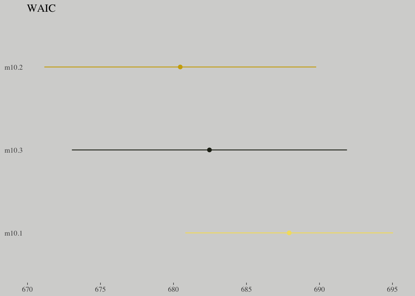
compare_ic(w_m10.10, w_m10.11, w_m10.12, w_m10.13, w_m10.14)## WAIC SE
## m10.10 80.16 11.83
## m10.11 79.20 11.68
## m10.12 84.56 9.43
## m10.13 150.70 47.42
## m10.14 141.53 33.51
## m10.10 - m10.11 0.96 1.31
## m10.10 - m10.12 -4.40 7.96
## m10.10 - m10.13 -70.55 47.33
## m10.10 - m10.14 -61.37 34.87
## m10.11 - m10.12 -5.36 8.38
## m10.11 - m10.13 -71.51 47.13
## m10.11 - m10.14 -62.33 34.65
## m10.12 - m10.13 -66.15 47.13
## m10.12 - m10.14 -56.97 33.35
## m10.13 - m10.14 9.17 17.07tibble(model = c("m10.10", "m10.11", "m10.12", "m10.13", "m10.14"),
waic = c(w_m10.10$estimates[3, 1], w_m10.11$estimates[3, 1], w_m10.12$estimates[3, 1], w_m10.13$estimates[3, 1], w_m10.14$estimates[3, 1]),
se = c(w_m10.10$estimates[3, 2], w_m10.11$estimates[3, 2], w_m10.12$estimates[3, 2], w_m10.13$estimates[3, 2], w_m10.14$estimates[3, 2])) %>%
ggplot() +
geom_pointrange(aes(x = reorder(model, -waic), y = waic,
ymin = waic - se,
ymax = waic + se,
color = model),
shape = 16) +
scale_color_manual(values = wes_palette("Moonrise2")[c(1, 2, 1, 1, 1)]) +
coord_flip() +
labs(x = NULL, y = NULL,
title = "WAIC") +
theme(axis.ticks.y = element_blank(),
legend.position = "none")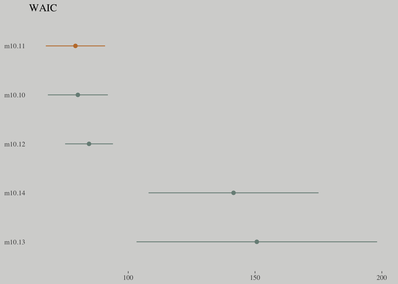
nd <-
    tibble(log_pop = rep(seq(from = 6.5,
                             to = 13,
                             length.out = 50),
                         times = 2),
           contact_high = rep(0:1, each = 50))

ppa_10.9 <-
    pp_average(m10.10, m10.11, m10.12,
               weights = "loo",
               method = "fitted",
               newdata = nd) %>%
    as_tibble() %>%
    bind_cols(nd)

ppa_10.9 %>%
    ggplot(aes(x = log_pop,
               group = contact_high)) +
    geom_ribbon(aes(ymin = `2.5%ile`,
                    ymax = `97.5%ile`,
                    fill = contact_high),
                alpha = 1/4) +
    geom_line(aes(y = Estimate, color = contact_high)) +
    geom_text(data = d,
              aes(y = total_tools,
                  label = total_tools,
                  color = contact_high),
              size = 3.5) +
    coord_cartesian(xlim = c(7.1, 12.4),
                    ylim = c(12, 70)) +
    labs(x = "log population",
         y = "total tools",
         subtitle = "Blue is the high contact rate and black is the low. Notice that both trends curve\n dramatically upwards as log-population increases. The impact of contact rate can be seen by the distance\n between the blue and gray predictions. There is plenty of overlap, especially at low and high\n log-population values, where there are no islands with high contact rate.") +
    theme(legend.position = "none",
          panel.border = element_blank())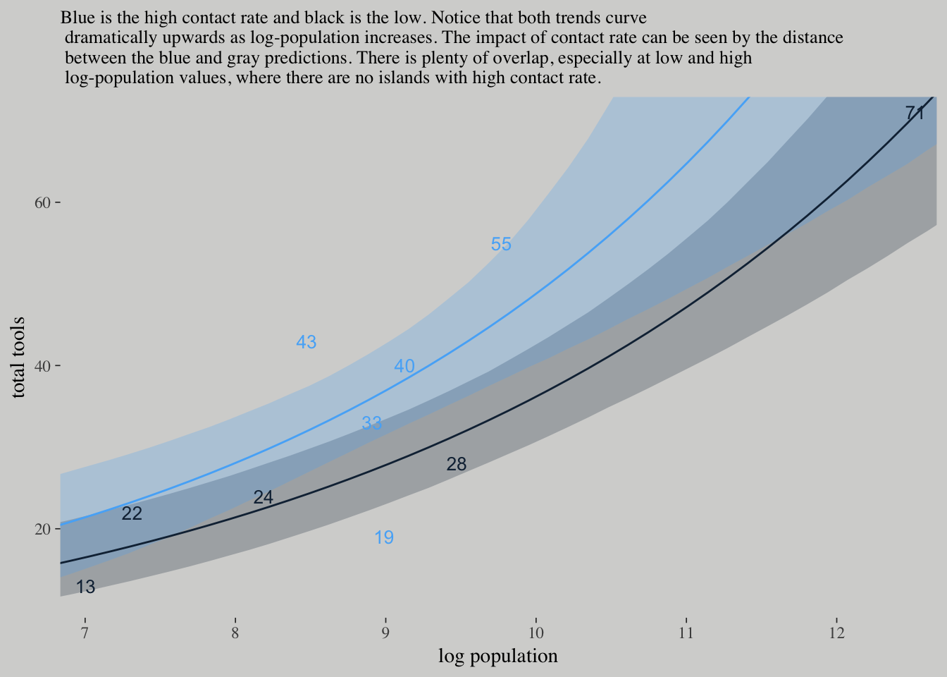
10.2.2. MCMC islands
d <-
    d %>%
    mutate(log_pop_c = log_pop - mean(log_pop))

m10.10.c <-
    brm(data = d, family = poisson,
        total_tools ~ 1 + log_pop_c + contact_high + contact_high:log_pop_c,
        prior = c(set_prior("normal(0, 10)", class = "Intercept"),
                  set_prior("normal(0, 10)", class = "b")),
        iter = 3000, warmup = 1000, chains = 4, cores = 4)
# this helps us set our custom color scheme
color_scheme_set(c(wes_palette("Moonrise2")[3],
wes_palette("Moonrise2")[1],
wes_palette("Moonrise2")[2],
wes_palette("Moonrise2")[2],
wes_palette("Moonrise2")[1],
wes_palette("Moonrise2")[1]))
# the actual plot
mcmc_pairs(x = posterior_samples(m10.10),
pars = c("b_Intercept", "b_log_pop", "b_contact_high", "b_log_pop:contact_high"),
off_diag_args = list(size = 1/10, alpha = 1/10),
diag_fun = "dens")## Warning in mcmc_pairs(x = posterior_samples(m10.10), pars =
## c("b_Intercept", : Only one chain in 'x'. This plot is more useful with
## multiple chains.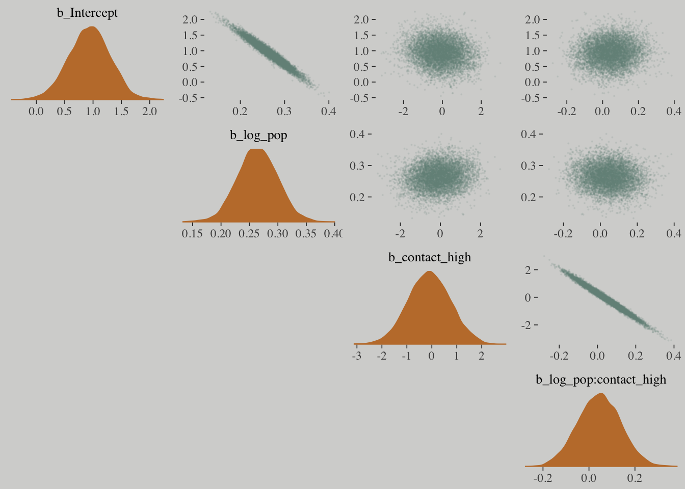
mcmc_pairs(x = posterior_samples(m10.10.c),
           pars = c("b_Intercept", "b_log_pop_c", "b_contact_high", "b_log_pop_c:contact_high"),
           off_diag_args = list(size = 1/10, alpha = 1/10),
           diag_fun = "dens")
## Warning in mcmc_pairs(x = posterior_samples(m10.10.c), pars =
## c("b_Intercept", : Only one chain in 'x'. This plot is more useful with
## multiple chains.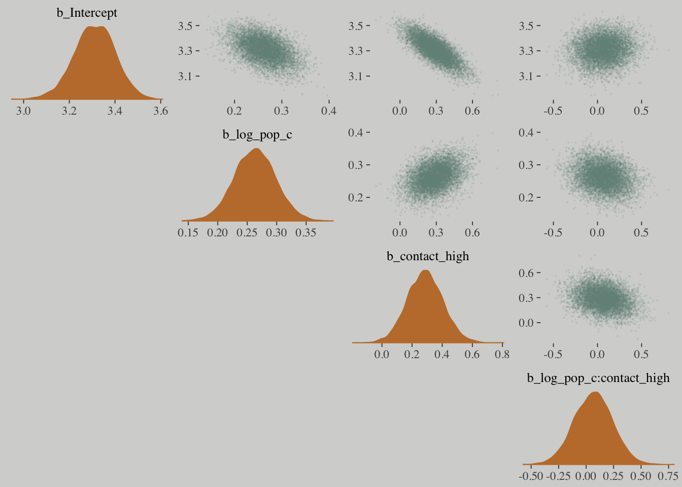
Hamiltonian Monte Carlo is very good at handling strong correlations in the posterior distribution, but it is going to be less efficient.
When strong correlations are gone, the Markov chain results in a greater number of effective samples.
Check the psych package for correlation matrices.
10.2.3. Example: Exposure and the offset
set.seed(3838) # making it reproducible

num_days <- 30
y <- rpois(num_days, 1.5)

set.seed(3838) # making it reproducible

num_weeks <- 4
y_new <- rpois(num_weeks, 0.5*7)

d <-
  tibble(y = c(y, y_new),
         days = c(rep(1, 30), rep(7, 4)),
         monastery = c(rep(0, 30), rep(1, 4)))

d
## # A tibble: 34 x 3
## y days monastery
## <int> <dbl> <dbl>
## 1 1 1. 0.
## 2 2 1. 0.
## 3 1 1. 0.
## 4 1 1. 0.
## 5 1 1. 0.
## 6 2 1. 0.
## 7 0 1. 0.
## 8 1 1. 0.
## 9 1 1. 0.
## 10 0 1. 0.
## # ... with 24 more rowsd <-
d %>%
mutate(log_days = log(days))
m10.15 <-
brm(data = d, family = poisson,
y ~ 1 + offset(log_days) + monastery,
prior = c(set_prior("normal(0, 100)", class = "Intercept"),
set_prior("normal(0, 1)", class = "b")),
iter = 2500, warmup = 500, cores = 2, chains = 2)We don’t use the offset again, when computing predictions, because the parameters are already on the same time scale.
posterior_samples(m10.15) %>%
    mutate(lambda_old = exp(b_Intercept),
           lambda_new  = exp(b_Intercept + b_monastery)) %>%
    gather(key, value, -(b_Intercept:lp__)) %>%
    mutate(key = factor(key, levels = c("lambda_old", "lambda_new"))) %>%
    group_by(key) %>%
    summarise(Mean = mean(value) %>% round(digits = 2),
              StdDev = sd(value) %>% round(digits = 2),
              LL = quantile(value, probs = .025) %>% round(digits = 2),
              UL = quantile(value, probs = .975) %>% round(digits = 2))
## # A tibble: 2 x 5
## key Mean StdDev LL UL
## <fct> <dbl> <dbl> <dbl> <dbl>
## 1 lambda_old 1.20 0.200 0.850 1.63
## 2 lambda_new 0.460 0.120 0.250 0.73010.3. Other count regressions
10.3.1. Multinomial
When more than two types of unordered events are possible, and the probability of each type of event is constant across trials, then the maximum entropy distribution is the multinomial distribution.
\[\Pr\left( { { y }_{ 1 }, \dots, { y }_{ K } }|{ n,{ { p }_{ 1 }, \dots, { p }_{ K } } } \right) =\frac { n! }{ \prod _{ i }{ { y }_{ i }! } } \prod _{ i=1 }^{ K }{ { p }_{ i }^{ { y }_{ i } } } \]
A model built on a multinomial distribution may also be called a categorical regression, usually when each event is isolated on a single row, like with logistic regression. In machine learning, this model type is sometimes known as the maximum entropy classifier.
10.3.1.1. Explicit multinomial models
This approach uses the multinomial likelihood and a generalization of the logit link (the multinomial logit).
The multinomial logit is a link function takes a vector of scores, one for each of \(K\) event types, and computes the probability of a particular type of event \(k\) as:
\[\Pr\left( { k }|{ { { s }_{ 1 }\dots { s }_{ K } } } \right) =\frac { exp\left( { s }_{ k } \right) }{ \sum _{ i=1 }^{ K }{ exp\left( { s }_{ i } \right) } } \]
Combined with this conventional link, this type of GLM is often called multinomial logistic regression.
In a binomial GLM, you can pick either of the two possible events and build a single linear model for its log odds. The other event is handled automatically. But in a multinomial (or categorical) GLM, you need \(K-1\) linear models for \(K\) types of events. In each of these, you can use any predictors and parameters you like (they don’t have to be the same, and there are often good reasons for them to be different). In the special case of two types of events, none of these choices arise, because there is only one linear model.
There are two basic cases: (1) predictors have different values for different types of events, and (2) parameters are distinct for each type of event. The first case is useful when each type of event has its own quantitative traits, and you want to estimate the association between those traits and the probability each type of event appears in the data. The second case is useful when you are interested instead in features of some entity that produces each event, whatever type it turns out to be.
detach(package:brms)
library(rethinking)
## rethinking (Version 1.59)##
## Attaching package: 'rethinking'## The following object is masked from 'package:loo':
##
## compare## The following object is masked from 'package:purrr':
##
## map# simulate career choices among 500 individuals
N <- 500 # number of individuals
income <- 1:3 # expected income of each career
score <- 0.5*income # scores for each career, based on income
# next line converts scores to probabilities
p <- softmax(score[1], score[2], score[3])
# now simulate choice
# outcome career holds event type values, not counts
career <- rep(NA, N) # empty vector of choices for each individual
set.seed(2078)
# sample chosen career for each individual
for(i in 1:N) career[i] <- sample(1:3, size = 1, prob = p)
career %>%
as_tibble() %>%
ggplot(aes(x = value %>% as.factor())) +
geom_bar(size = 0, fill = wes_palette("Moonrise2")[2])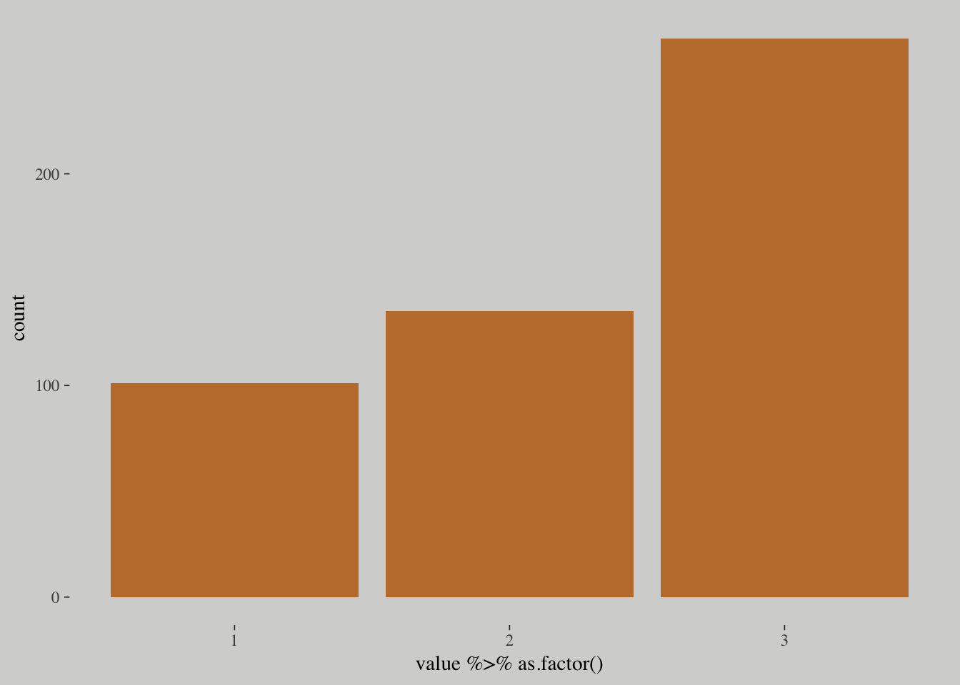
detach(package:rethinking)
library(brms)

m10.16 <-
    brm(data = list(career = career),
        family = categorical(link = "logit"),
        career ~ 1,
        prior = c(set_prior("normal(0, 5)", class = "Intercept")),
        iter = 2500, warmup = 500, cores = 2, chains = 2)

print(m10.16)
## Family: categorical
## Links: mu2 = logit; mu3 = logit
## Formula: career ~ 1
## Data: list(career = career) (Number of observations: 500)
## Samples: 2 chains, each with iter = 2500; warmup = 500; thin = 1;
## total post-warmup samples = 4000
## ICs: LOO = NA; WAIC = NA; R2 = NA
##
## Population-Level Effects:
## Estimate Est.Error l-95% CI u-95% CI Eff.Sample Rhat
## mu2_Intercept 0.29 0.13 0.04 0.55 1374 1.00
## mu3_Intercept 0.96 0.12 0.73 1.20 1403 1.00
##
## Samples were drawn using sampling(NUTS). For each parameter, Eff.Sample
## is a crude measure of effective sample size, and Rhat is the potential
## scale reduction factor on split chains (at convergence, Rhat = 1).Be aware that the estimates you get from these models are extraordinarily difficult to interpret. You absolutely must convert them to a vector of probabilities, to make much sense of them. The principle reason is that the estimates swing around wildly, depending upon which event type you assign a constant score.
Have a look at this blog post for an understanding of multinomial logistic regression models.
library(rethinking)

N <- 100

set.seed(2078)
# simulate family incomes for each individual
family_income <- runif(N)

# assign a unique coefficient for each type of event
b <- (1:-1)
career <- rep(NA, N)  # empty vector of choices for each individual

for (i in 1:N) {
    score <- 0.5*(1:3) + b*family_income[i]
    p <- softmax(score[1], score[2], score[3])
    career[i] <- sample(1:3, size = 1, prob = p)
}
detach(package:rethinking)
library(brms)
m10.17 <-
brm(data = list(career = career,
family_income = family_income),
family = categorical(link = "logit"),
career ~ 1 + family_income,
prior = c(set_prior("normal(0, 5)", class = "Intercept"),
set_prior("normal(0, 5)", class = "b")),
iter = 2500, warmup = 500, cores = 2, chains = 2)
print(m10.17)## Family: categorical
## Links: mu2 = logit; mu3 = logit
## Formula: career ~ 1 + family_income
## Data: list(career = career, family_income = family_incom (Number of observations: 100)
## Samples: 2 chains, each with iter = 2500; warmup = 500; thin = 1;
## total post-warmup samples = 4000
## ICs: LOO = NA; WAIC = NA; R2 = NA
##
## Population-Level Effects:
## Estimate Est.Error l-95% CI u-95% CI Eff.Sample Rhat
## mu2_Intercept 1.86 0.58 0.76 3.04 2281 1.00
## mu3_Intercept 1.54 0.57 0.48 2.73 2265 1.00
## mu2_family_income -3.96 1.05 -6.16 -2.02 2762 1.00
## mu3_family_income -2.55 0.94 -4.49 -0.81 2745 1.00
##
## Samples were drawn using sampling(NUTS). For each parameter, Eff.Sample
## is a crude measure of effective sample size, and Rhat is the potential
## scale reduction factor on split chains (at convergence, Rhat = 1).10.3.1.2. Multinomial in disguise as Poisson
Another way to fit a multinomial likelihood is to refactor it into a series of Poisson likelihoods
library(rethinking)

data(UCBadmit)
d <- UCBadmit
rm(UCBadmit)

detach(package:rethinking)
library(brms)
## Warning: package 'brms' was built under R version 3.4.4# binomial model of overall admission probability
m_binom <-
brm(data = d, family = binomial,
admit | trials(applications) ~ 1,
prior = c(set_prior("normal(0, 100)", class = "Intercept")),
iter = 2000, warmup = 1000, cores = 3, chains = 3)
# Poisson model of overall admission rate and rejection rate
d <-
d %>%
mutate(rej = reject) # 'reject' is a reserved word
m_pois <-
brm(data = d, family = poisson,
cbind(admit, rej) ~ 1,
prior = c(set_prior("normal(0, 100)", class = "Intercept")),
iter = 2000, warmup = 1000, cores = 3, chains = 3)
print(m_pois)## Family: MV(poisson, poisson)
## Links: mu = log
## mu = log
## Formula: admit ~ 1
## rej ~ 1
## Data: d (Number of observations: 12)
## Samples: 3 chains, each with iter = 2000; warmup = 1000; thin = 1;
## total post-warmup samples = 3000
## ICs: LOO = NA; WAIC = NA; R2 = NA
##
## Population-Level Effects:
## Estimate Est.Error l-95% CI u-95% CI Eff.Sample Rhat
## admit_Intercept 4.99 0.02 4.94 5.03 2205 1.00
## rej_Intercept 5.44 0.02 5.41 5.48 2084 1.00
##
## Samples were drawn using sampling(NUTS). For each parameter, Eff.Sample
## is a crude measure of effective sample size, and Rhat is the potential
## scale reduction factor on split chains (at convergence, Rhat = 1).posterior_samples(m_pois) %>%
ggplot(aes(x = exp(b_admit_Intercept))) +
geom_density(fill = wes_palette("Moonrise2")[2], size = 0) +
geom_vline(xintercept = mean(d$admit), color = wes_palette("Moonrise2")[1]) +
scale_y_continuous(NULL, breaks = NULL) +
labs(x = "# applications",
title = "Mean acceptance # across departments:",
subtitle = "The density is the posterior distribution. The line is the\nvalue in the data.")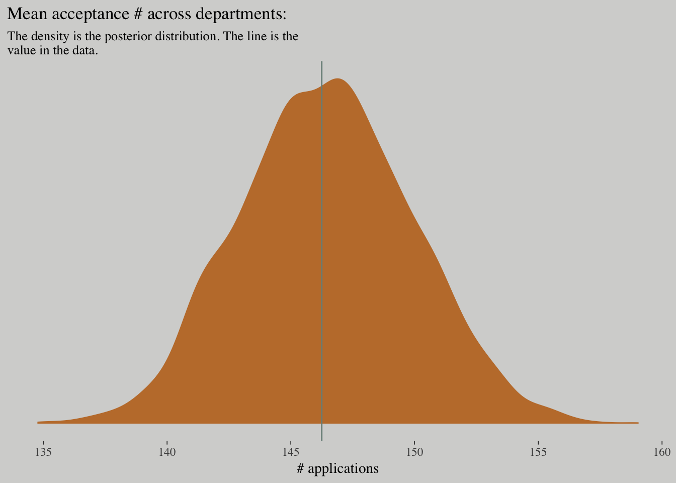
posterior_samples(m_pois) %>%
    ggplot(aes(x = exp(b_rej_Intercept))) +
    geom_density(fill = wes_palette("Moonrise2")[1], size = 0) +
    geom_vline(xintercept = mean(d$rej), color = wes_palette("Moonrise2")[2]) +
    scale_y_continuous(NULL, breaks = NULL) +
    labs(x = "# applications",
         title = "Mean rejection # across departments:",
         subtitle = "The density is the posterior distribution. The line is the\nvalue in the data.")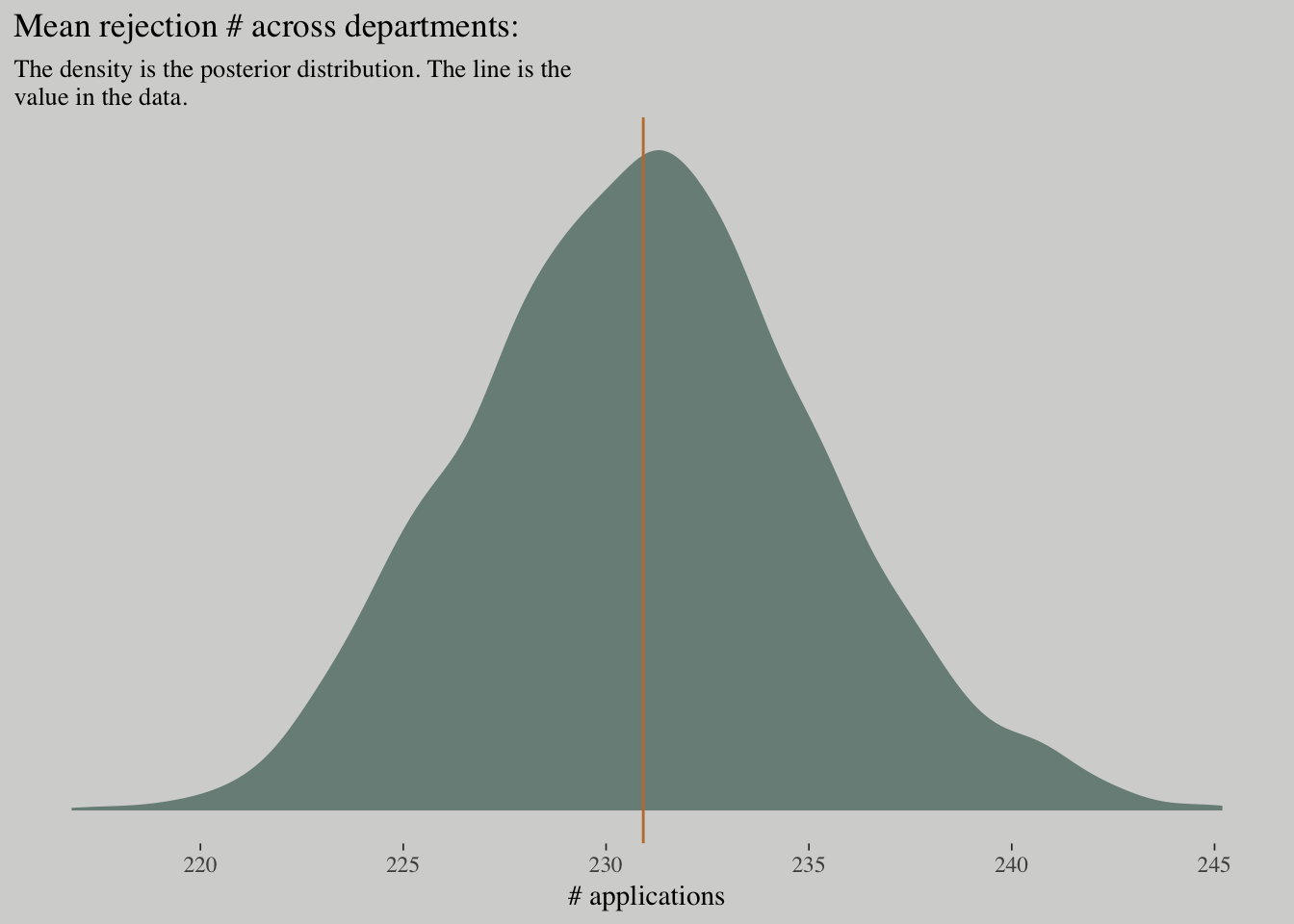
fixef(m_binom) %>%
  invlogit()
## Estimate Est.Error 2.5%ile 97.5%ile
## Intercept 0.3876835 0.5076754 0.3732773 0.4020179k <-
fixef(m_pois) %>%
as.numeric()
exp(k[1])/(exp(k[1]) + exp(k[2]))## [1] 0.3880054Have a look at Estimating Multivariate Models with brms.
10.3.2. Geometric
Sometimes a count variable is a number of events up until something happened. Call this “something” the terminating event. Often we want to model the probability of that event, a kind of analysis known as event history analysis or survival analysis. When the probability of the terminating event is constant through time (or distance), and the units of time (or distance) are discrete, a common likelihood function is the geometric distribution. This distribution has the form:
\[\Pr \left(y | p\right) = p \left( 1-p \right)^{y-1}\]
The geometric distribution has maximum entropy for unbounded counts with constant expected value.
# simulate
N <- 100
set.seed(1028)
x <- runif(N)

set.seed(1028)
y <- rgeom(N, prob = invlogit(-1 + 2*x))

list(y = y, x = x) %>%
    as_tibble() %>%
    ggplot(aes(x = x, y = y)) +
    geom_point(size = 3/5, alpha = 2/3)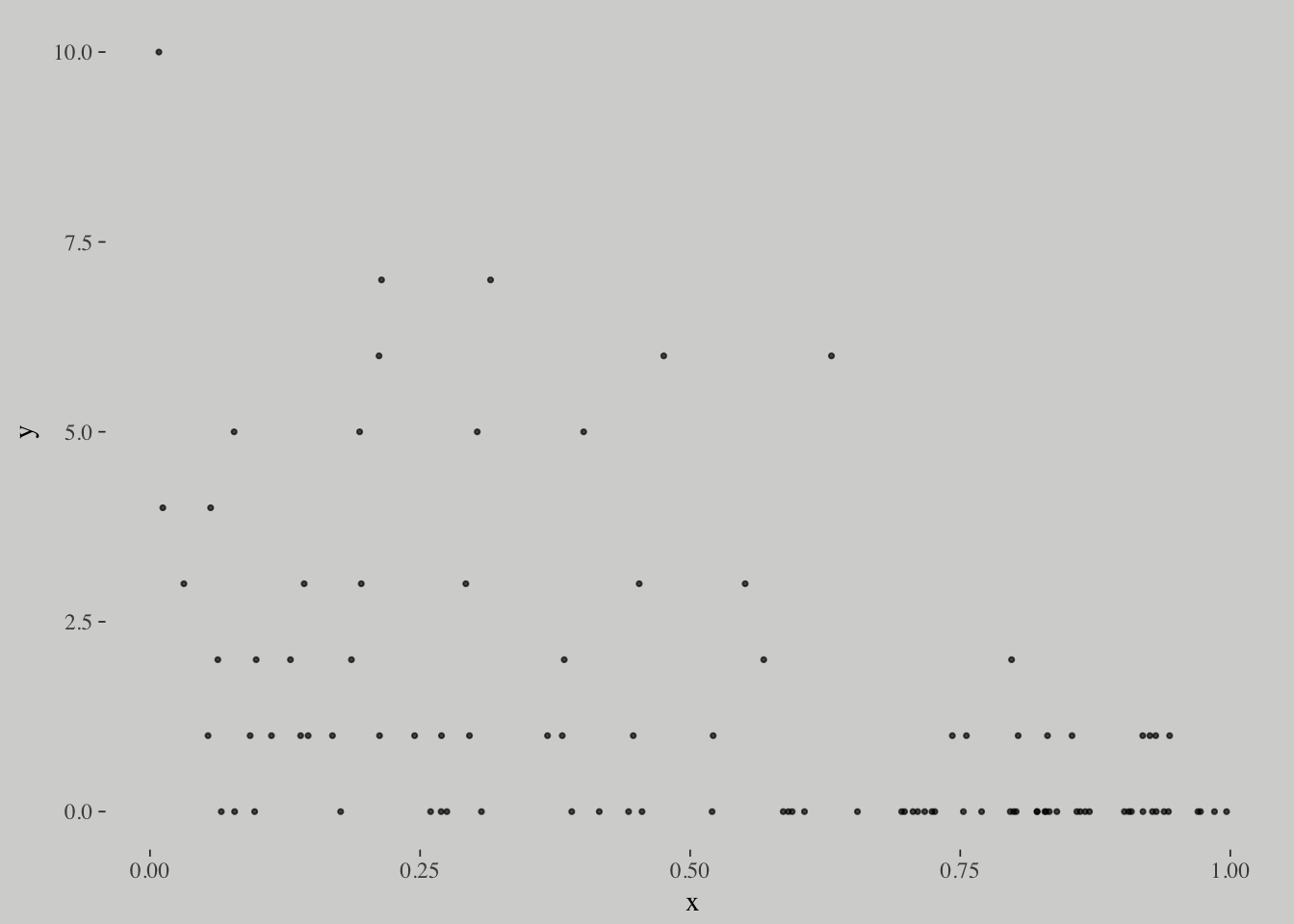
m10.18 <-
    brm(data = list(y = y, x = x),
        family = geometric(link = "log"),
        y ~ 0 + intercept + x,
        prior = c(set_prior("normal(0, 10)", class = "b", coef = "intercept"),
                  set_prior("normal(0, 1)", class = "b")),
        chains = 2, iter = 2500, warmup = 500, cores = 2)

print(m10.18)
## Family: geometric
## Links: mu = log
## Formula: y ~ 0 + intercept + x
## Data: list(y = y, x = x) (Number of observations: 100)
## Samples: 2 chains, each with iter = 2500; warmup = 500; thin = 1;
## total post-warmup samples = 4000
## ICs: LOO = NA; WAIC = NA; R2 = NA
##
## Population-Level Effects:
## Estimate Est.Error l-95% CI u-95% CI Eff.Sample Rhat
## intercept 1.16 0.23 0.72 1.60 1228 1.00
## x -2.28 0.44 -3.19 -1.46 1207 1.00
##
## Samples were drawn using sampling(NUTS). For each parameter, Eff.Sample
## is a crude measure of effective sample size, and Rhat is the potential
## scale reduction factor on split chains (at convergence, Rhat = 1).plot(marginal_effects(m10.18),
points = T,
point_args = c(size = 3/5, alpha = 2/3),
line_args = c(color = wes_palette("Moonrise2")[1],
fill = wes_palette("Moonrise2")[1]))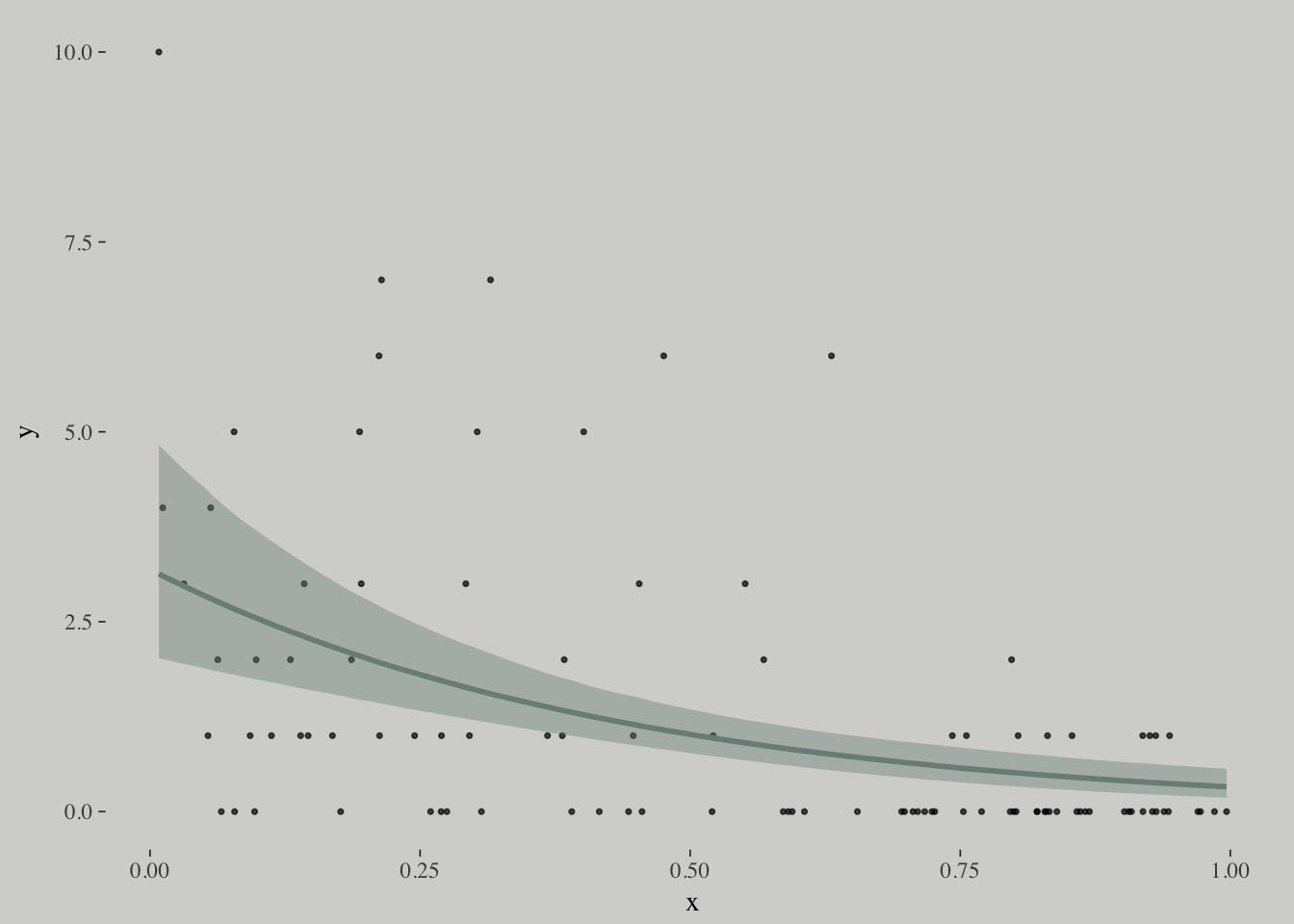
References
McElreath, R. (2016). Statistical rethinking: A Bayesian course with examples in R and Stan. Chapman & Hall/CRC Press.
Kurz, A. S. (2018, March 9). brms, ggplot2 and tidyverse code, by chapter. Retrieved from https://goo.gl/JbvNTj
