Mixture modeling help us transform our modeling to cope with the inconvenient realities of measurement, rather than transforming measurements to cope with the constraints of our models.
11.1. Ordered categorical outcomes
It is very common in the social sciences, and occasional in the natural sciences, to have an outcome variable that is discrete, like a count, but in which the values merely indicate different ordered levels along some dimension. But unlike a count, the differences in value are not necessarily equal.
An ordered categorical variable is just a multinomial prediction problem. But the constraint that the categories be ordered demands a special treatment. What we’d like is for any associated predictor variable, as it increases, to move predictions progressively through the categories in sequence. The conventional solution is to use a cumulative link function.
By linking a linear model to cumulative probability, it is possible to guarantee the ordering of the outcomes.
11.1.1. Example: Moral intuition
library(rethinking)
data(Trolley)
d <- Trolley

rm(Trolley)
detach(package:rethinking, unload = T)
library(brms)

library(ggthemes)
scales::show_col(canva_pal("Green fields")(4))
11.1.2. Describing an ordered distribution with intercepts
library(tidyverse)## ── Attaching packages ──────────────────────────────────────────────────────────────────── tidyverse 1.2.1 ──## ✔ tibble 1.4.2 ✔ purrr 0.2.5
## ✔ tidyr 0.8.1 ✔ dplyr 0.7.5
## ✔ readr 1.1.1 ✔ stringr 1.3.1
## ✔ tibble 1.4.2 ✔ forcats 0.3.0## ── Conflicts ─────────────────────────────────────────────────────────────────────── tidyverse_conflicts() ──
## ✖ tidyr::extract() masks rstan::extract()
## ✖ dplyr::filter() masks stats::filter()
## ✖ dplyr::lag() masks stats::lag()hist_plot <- ggplot(data = d, aes(x = response, fill = ..x..)) +
geom_histogram(binwidth = 1/4, size = 0) +
scale_x_continuous(breaks = 1:7) +
theme_hc() +
scale_fill_gradient(low = canva_pal("Green fields")(4)[4],
high = canva_pal("Green fields")(4)[1]) +
theme(axis.ticks.x = element_blank(),
plot.background = element_rect(fill = "grey92"),
legend.position = "none")
cum_plot <- d %>%
group_by(response) %>%
count() %>%
mutate(pr_k = n/nrow(d)) %>%
ungroup() %>%
mutate(cum_pr_k = cumsum(pr_k)) %>%
ggplot(aes(x = response, y = cum_pr_k,
fill = response)) +
geom_line(color = canva_pal("Green fields")(4)[2]) +
geom_point(shape = 21, colour = "grey92",
size = 2.5, stroke = 1) +
scale_x_continuous(breaks = 1:7) +
scale_y_continuous(breaks = c(0, .5, 1)) +
coord_cartesian(ylim = c(0, 1)) +
labs(y = "cumulative proportion") +
theme_hc() +
scale_fill_gradient(low = canva_pal("Green fields")(4)[4],
high = canva_pal("Green fields")(4)[1]) +
theme(axis.ticks.x = element_blank(),
plot.background = element_rect(fill = "grey92"),
legend.position = "none")
# McElreath's convenience function
logit <- function(x) log(x/(1-x))
log_cum_odd_plot <- d %>%
group_by(response) %>%
count() %>%
mutate(pr_k = n/nrow(d)) %>%
ungroup() %>%
mutate(cum_pr_k = cumsum(pr_k)) %>%
filter(response < 7) %>%
# We can do the logit() conversion right in ggplot2
ggplot(aes(x = response, y = logit(cum_pr_k),
fill = response)) +
geom_line(color = canva_pal("Green fields")(4)[2]) +
geom_point(shape = 21, colour = "grey92",
size = 2.5, stroke = 1) +
scale_x_continuous(breaks = 1:7) +
coord_cartesian(xlim = c(1, 7)) +
labs(y = "log-cumulative-odds") +
theme_hc() +
scale_fill_gradient(low = canva_pal("Green fields")(4)[4],
high = canva_pal("Green fields")(4)[1]) +
theme(axis.ticks.x = element_blank(),
plot.background = element_rect(fill = "grey92"),
legend.position = "none")
library(gridExtra)##
## Attaching package: 'gridExtra'## The following object is masked from 'package:dplyr':
##
## combinegrid.arrange(hist_plot, cum_plot, log_cum_odd_plot, ncol=3)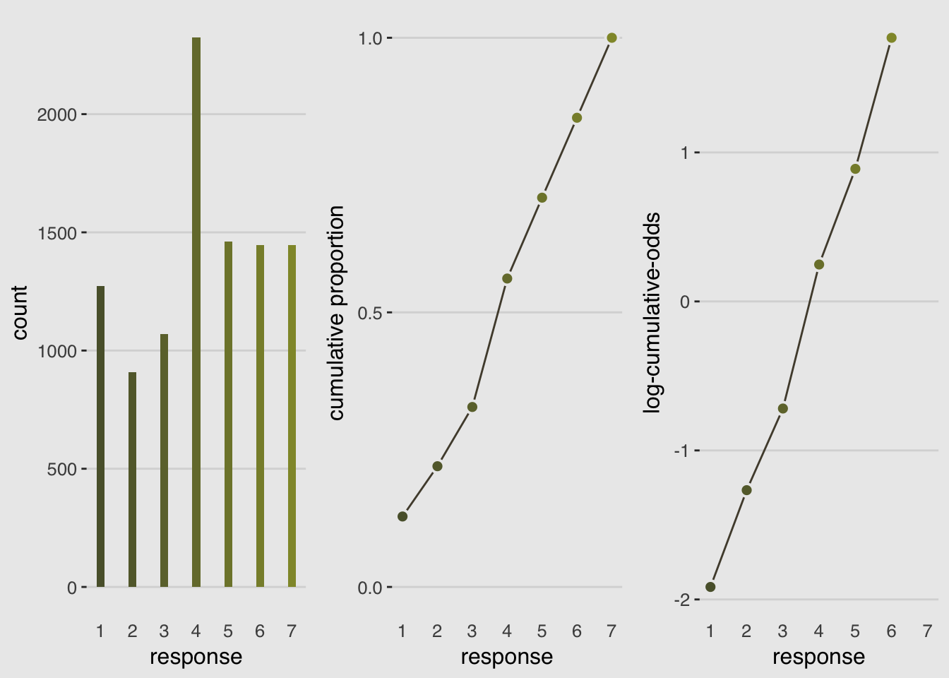
d_plot <-
    d %>%
    group_by(response) %>%
    count() %>%
    mutate(pr_k = n/nrow(d)) %>%
    ungroup() %>%
    mutate(cum_pr_k = cumsum(pr_k))

ggplot(data = d_plot,
       aes(x = response, y = cum_pr_k,
           color = cum_pr_k, fill = cum_pr_k)) +
    geom_line(color = canva_pal("Green fields")(4)[1]) +
    geom_point(shape = 21, colour = "grey92",
               size = 2.5, stroke = 1) +
    geom_linerange(aes(ymin = 0, ymax = cum_pr_k),
                   alpha = 1/2, color = canva_pal("Green fields")(4)[1]) +
    # There are probably more elegant ways to do this part.
    geom_linerange(data = . %>%
                       mutate(discrete_probability = ifelse(response == 1, cum_pr_k, cum_pr_k - pr_k)),
                   aes(x = response + .025,
                       ymin = ifelse(response == 1, 0, discrete_probability),
                       ymax = cum_pr_k),
                   color = "black") +
    geom_text(data = tibble(text = 1:7,
                            response = seq(from = 1.25, to = 7.25, by = 1),
                            cum_pr_k = d_plot$cum_pr_k - .065),
              aes(label = text),
              size = 4) +
    scale_x_continuous(breaks = 1:7) +
    scale_y_continuous(breaks = c(0, .5, 1)) +
    coord_cartesian(ylim = c(0, 1)) +
    labs(y = "cumulative proportion") +
    theme_hc() +
    scale_fill_gradient(low = canva_pal("Green fields")(4)[4],
                        high = canva_pal("Green fields")(4)[1]) +
    scale_color_gradient(low = canva_pal("Green fields")(4)[4],
                         high = canva_pal("Green fields")(4)[1]) +
    theme(axis.ticks.x = element_blank(),
          plot.background = element_rect(fill = "grey92"),
          legend.position = "none")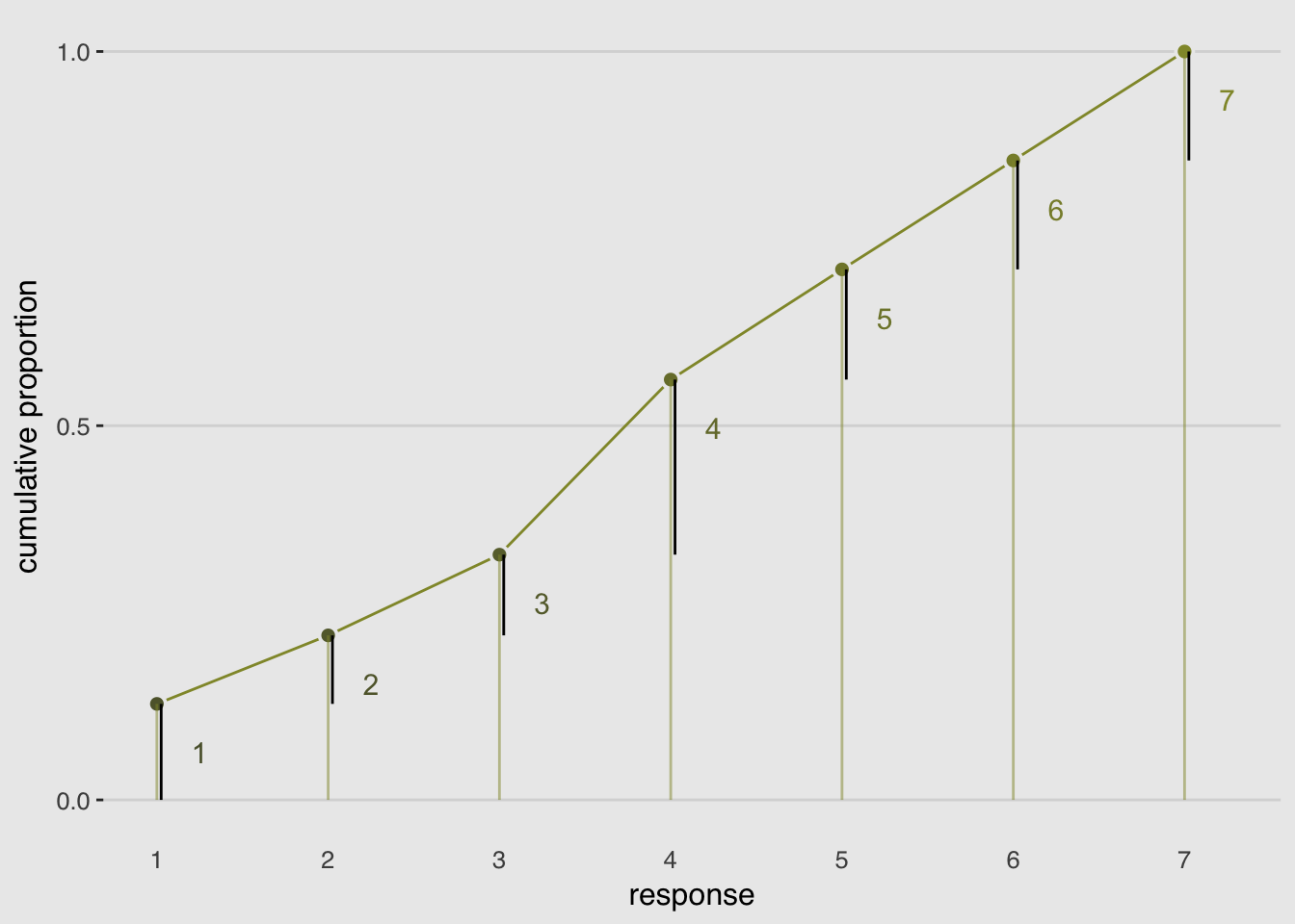
The model is defined as:
\[\begin{eqnarray} { R }_{ i } & \sim & \text{Ordered}\left( \mathbf{p} \right) \\ \text{logit} \left( \Pr \left( R_i \le k \right) \right) & = & \alpha_k \end{eqnarray}\]
Notice that the cumulative logit of the largest response is infinity.
# Here are our starting values, which we specify with the `inits` argument in brm()
Inits <- list(`Intercept[1]` = -2,
              `Intercept[2]` = -1,
              `Intercept[3]` = 0,
              `Intercept[4]` = 1,
              `Intercept[5]` = 2,
              `Intercept[6]` = 2.5)

InitsList <-list(Inits, Inits)

m11.1 <-
    brm(data = d, family = cumulative,
        response ~ 1,
        prior = c(set_prior("normal(0, 10)", class = "Intercept")),
        iter = 2000, warmup = 1000, cores = 2, chains = 2,
        inits = InitsList)  # Here we place our start values into brm()

print(m11.1)
## Family: cumulative
## Links: mu = logit; disc = identity
## Formula: response ~ 1
## Data: d (Number of observations: 9930)
## Samples: 2 chains, each with iter = 2000; warmup = 1000; thin = 1;
## total post-warmup samples = 2000
## ICs: LOO = NA; WAIC = NA; R2 = NA
##
## Population-Level Effects:
## Estimate Est.Error l-95% CI u-95% CI Eff.Sample Rhat
## Intercept[1] -1.92 0.03 -1.98 -1.86 1528 1.00
## Intercept[2] -1.27 0.02 -1.31 -1.22 2000 1.00
## Intercept[3] -0.72 0.02 -0.76 -0.68 2000 1.00
## Intercept[4] 0.25 0.02 0.21 0.29 2000 1.00
## Intercept[5] 0.89 0.02 0.85 0.94 2000 1.00
## Intercept[6] 1.77 0.03 1.71 1.83 2000 1.00
##
## Samples were drawn using sampling(NUTS). For each parameter, Eff.Sample
## is a crude measure of effective sample size, and Rhat is the potential
## scale reduction factor on split chains (at convergence, Rhat = 1).invlogit <- function(x) {1/(1+exp(-x))}
m11.1 %>%
fixef() %>%
invlogit()## Estimate Est.Error Q2.5 Q97.5
## Intercept[1] 0.1282493 0.5075149 0.1218421 0.1350510
## Intercept[2] 0.2196851 0.5061199 0.2117017 0.2281557
## Intercept[3] 0.3276420 0.5053175 0.3188293 0.3371890
## Intercept[4] 0.5617552 0.5050194 0.5522268 0.5714108
## Intercept[5] 0.7090390 0.5056345 0.7002370 0.7181145
## Intercept[6] 0.8545451 0.5070798 0.8474365 0.861270011.1.3. Adding predictor variables
To include predictor variables, we define the log-cumulative-odds of each response \(k\) as a sum of its intercept \(\alpha_k\) and a typical linear model \(\phi_i\).
\[\begin{eqnarray} { R }_{ i } & \sim & \text{Ordered}\left( \mathbf{p} \right) \\ \text{logit} \left( \Pr \left( R_i \le k \right) \right) & = & \alpha_k - \phi_i \end{eqnarray}\]
where \(\phi_i = \beta x_i\)
Why is the linear model \(\phi\) subtracted from each intercept? Because if we decrease the log-cumulative odds of every outcome value \(k\) below the maximum, this necessarily shifts probability mass upwards towards higher outcome values.
# First, we needed to specify the logistic() function, which is apart of the dordlogit() function
logistic <- function(x) {
    p <- 1 / (1 + exp(-x))
    p <- ifelse(x == Inf, 1, p)
    p
}

# Now we get down to it
dordlogit <- function(x, phi, a, log = FALSE) {
    a  <- c(as.numeric(a), Inf)
    p  <- logistic(a[x] - phi)
    na <- c(-Inf, a)
    np <- logistic(na[x] - phi)
    p  <- p - np
    if (log == TRUE) p <- log(p)
    p
}
pk <- dordlogit(1:7, 0, fixef(m11.1)[, 1])
pk## [1] 0.12824925 0.09143585 0.10795693 0.23411314 0.14728381 0.14550606
## [7] 0.14545495pk <- dordlogit(1:7, 0.5, fixef(m11.1)[, 1])
pk## [1] 0.08192101 0.06393219 0.08228230 0.20926676 0.15905405 0.18440673
## [7] 0.21913697# Start values for b11.2
Inits <- list(`Intercept[1]` = -1.9,
`Intercept[2]` = -1.2,
`Intercept[3]` = -0.7,
`Intercept[4]` = 0.2,
`Intercept[5]` = 0.9,
`Intercept[6]` = 1.8,
action = 0,
intention = 0,
contact = 0)
m11.2 <-
brm(data = d, family = cumulative,
response ~ 1 + action + intention + contact,
prior = c(set_prior("normal(0, 10)", class = "Intercept"),
set_prior("normal(0, 10)", class = "b")),
iter = 2000, warmup = 1000, cores = 2, chains = 2,
inits = list(Inits, Inits))
# Start values for b11.3
Inits <- list(`Intercept[1]` = -1.9,
`Intercept[2]` = -1.2,
`Intercept[3]` = -0.7,
`Intercept[4]` = 0.2,
`Intercept[5]` = 0.9,
`Intercept[6]` = 1.8,
action = 0,
intention = 0,
contact = 0,
`action:intention` = 0,
`contact:intention` = 0)
m11.3 <-
brm(data = d, family = cumulative,
response ~ 1 + action + intention + contact + action:intention + contact:intention,
prior = c(set_prior("normal(0, 10)", class = "Intercept"),
set_prior("normal(0, 10)", class = "b")),
iter = 2000, warmup = 1000, cores = 2, chains = 2,
inits = list(Inits, Inits))library(broom)
tidy(m11.1) %>% mutate(model = "m11.1") %>%
bind_rows(tidy(m11.2) %>% mutate(model = "m11.2")) %>%
bind_rows(tidy(m11.3) %>% mutate(model = "m11.3")) %>%
select(model, term, estimate) %>%
filter(term != "lp__") %>%
complete(term = distinct(., term), model) %>%
mutate(estimate = round(estimate, digits = 2)) %>%
spread(key = model, value = estimate) %>%
slice(c(6:11, 1, 4, 3, 2, 5)) # Here we indicate the order we'd like the rows in## term m11.1 m11.2 m11.3
## 1 b_Intercept[1] -1.92 -2.84 -2.64
## 2 b_Intercept[2] -1.27 -2.16 -1.94
## 3 b_Intercept[3] -0.72 -1.57 -1.34
## 4 b_Intercept[4] 0.25 -0.55 -0.31
## 5 b_Intercept[5] 0.89 0.12 0.36
## 6 b_Intercept[6] 1.77 1.02 1.27
## 7 b_action NA -0.71 -0.47
## 8 b_intention NA -0.72 -0.28
## 9 b_contact NA -0.96 -0.33
## 10 b_action:intention NA NA -0.44
## 11 b_intention:contact NA NA -1.27loo::compare(waic(m11.1), waic(m11.2), waic(m11.3))## elpd_diff se_diff elpd_waic p_waic waic
## waic(m11.3) 0.0 0.0 -18464.7 11.1 36929.3
## waic(m11.2) -80.3 12.8 -18545.0 9.1 37090.0
## waic(m11.1) -462.6 31.3 -18927.2 6.0 37854.5nd <-
tibble(action = 0,
contact = 0,
intention = 0:1)
max_iter <- 100
fitted(m11.3,
newdata = nd,
subset = 1:max_iter,
summary = F) %>%
as_tibble() %>%
# We convert the data to the long format
gather() %>%
# We need an variable to index which posterior iteration we're working with
mutate(iter = rep(1:max_iter, times = 14)) %>%
# This step isn’t technically necessary, but I prefer my iter index at the far left.
select(iter, everything()) %>%
# Here we extract the `intention` and `response` information out of the `key` vector and spread it into two vectors.
separate(key, into = c("intention", "rating")) %>%
# That step produced two character vectors. They’ll be more useful as numbers
mutate(intention = intention %>% as.double(),
rating = rating %>% as.double()) %>%
# Here we convert `intention` into its proper 0:1 metric
mutate(intention = intention -1) %>%
# This isn't necessary, but it helps me understand exactly what metric the values are currently in
rename(pk = value) %>%
# This step is based on McElreath's R code 11.10 on page 338
mutate(`pk:rating` = pk*rating) %>%
# I’m not sure how to succinctly explain this. You’re just going to have to trust me.
group_by(iter, intention) %>%
# This is very important for the next step.
arrange(iter, intention, rating) %>%
# Here we take our `pk` values and make culmulative sums. Why? Take a long hard look at Figure 11.2.
mutate(probability = cumsum(pk)) %>%
# `rating == 7` is unnecessary. These `probability` values are by definition 1.
filter(rating < 7) %>%
ggplot(aes(x = intention,
y = probability,
color = probability)) +
geom_line(aes(group = interaction(iter, rating)),
alpha = 1/10) +
# Note how we made a new data object for geom_text()
geom_text(data = tibble(text = 1:7,
intention = seq(from = .9, to = .1, length.out = 7),
probability = c(.05, .12, .20, .35, .53, .71, .87)),
aes(label = text),
size = 3) +
scale_x_continuous(breaks = 0:1) +
scale_y_continuous(breaks = c(0, .5, 1)) +
coord_cartesian(ylim = 0:1) +
labs(subtitle = "action = 0,\ncontact = 0",
x = "intention") +
theme_hc() +
scale_color_gradient(low = canva_pal("Green fields")(4)[4],
high = canva_pal("Green fields")(4)[1]) +
theme(plot.background = element_rect(fill = "grey92"),
legend.position = "none")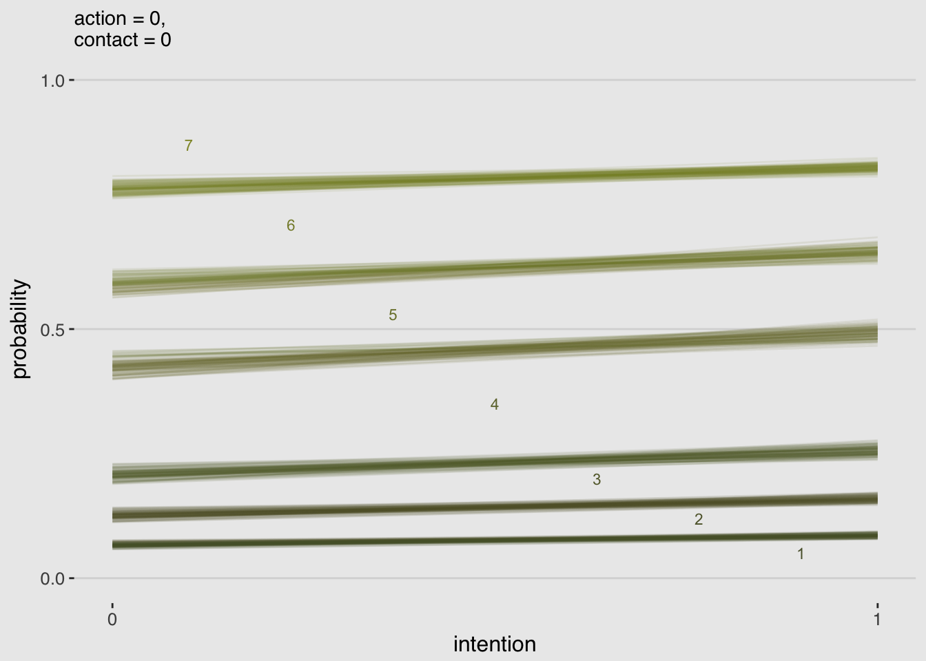
make_data_for_an_alternative_fiture <- function(action, contact, max_iter){

  nd <-
    tibble(action = action,
           contact = contact,
           intention = 0:1)

  max_iter <- max_iter

  fitted(m11.3,
         newdata = nd,
         subset = 1:max_iter,
         summary = F) %>%
    as_tibble() %>%
    gather() %>%
    mutate(iter = rep(1:max_iter, times = 14)) %>%
    select(iter, everything()) %>%
    separate(key, into = c("intention", "rating")) %>%
    mutate(intention = intention %>% as.double(),
           rating =  rating %>% as.double()) %>%
    mutate(intention = intention -1) %>%
    rename(pk = value) %>%
    mutate(`pk:rating` = pk*rating) %>%
    group_by(iter, intention) %>%

    # Everything above this point is identical to the previous custom function.
    # All we do is replace the last few lines with this one line of code.
    summarise(mean_rating = sum(`pk:rating`))
}
# Alternative to Figure 11.3.a
make_data_for_an_alternative_fiture(action = 0,
contact = 0,
max_iter = 100) %>%
ggplot(aes(x = intention, y = mean_rating, group = iter)) +
geom_line(alpha = 1/10, color = canva_pal("Green fields")(4)[1]) +
scale_x_continuous(breaks = 0:1) +
scale_y_continuous(breaks = 1:7) +
coord_cartesian(ylim = 1:7) +
labs(subtitle = "action = 0,\ncontact = 0",
x = "intention",
y = "response") +
theme_hc() +
theme(plot.background = element_rect(fill = "grey92"),
legend.position = "none")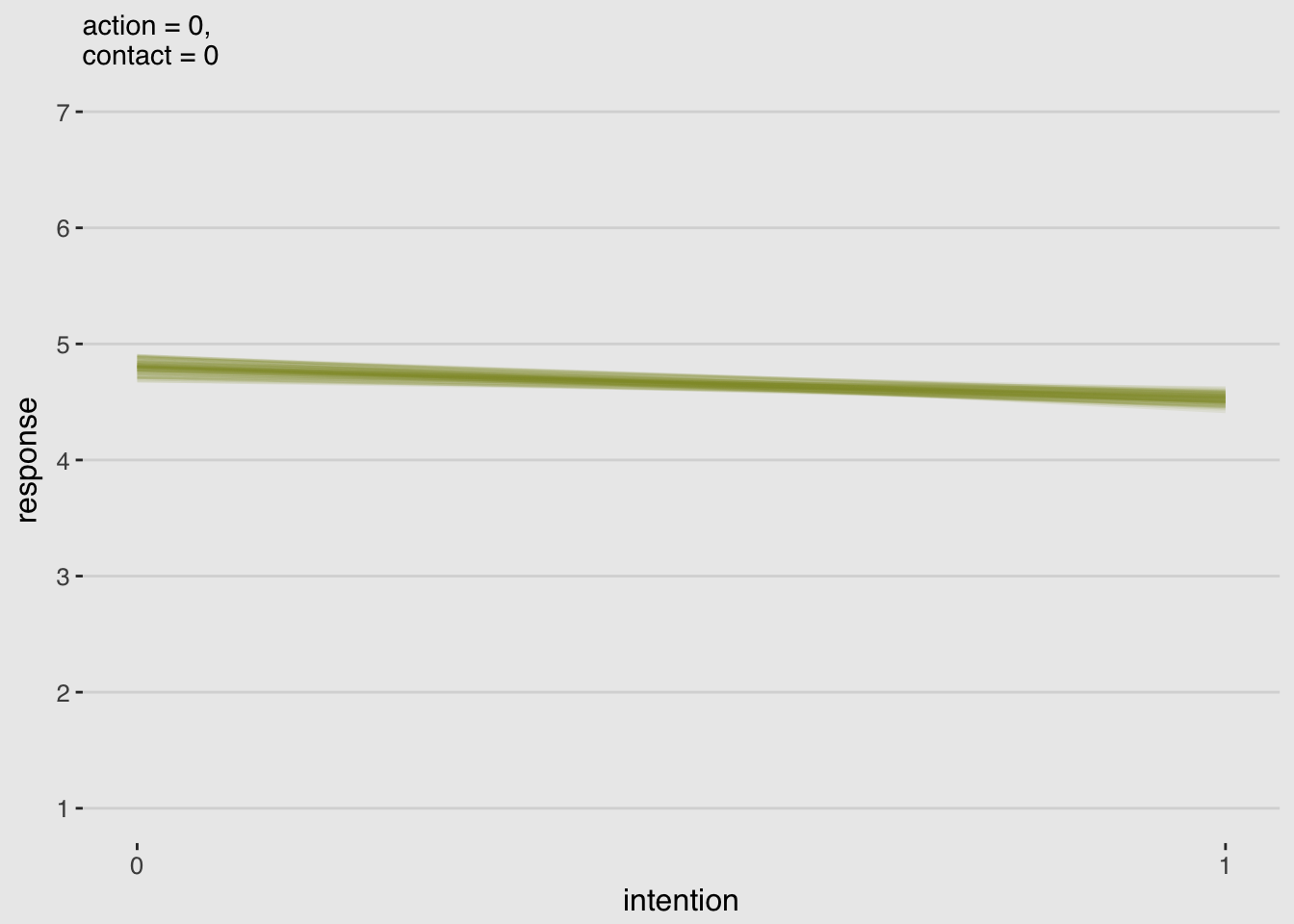
# Alternative to Figure 11.3.b
make_data_for_an_alternative_fiture(action = 1,
                                    contact = 0,
                                    max_iter = 100) %>%

 ggplot(aes(x = intention, y = mean_rating, group = iter)) +
  geom_line(alpha = 1/10, color = canva_pal("Green fields")(4)[1]) +
  scale_x_continuous(breaks = 0:1) +
  scale_y_continuous(breaks = 1:7) +
  coord_cartesian(ylim = 1:7) +
  labs(subtitle = "action = 1,\ncontact = 0",
       x = "intention",
       y = "response") +
  theme_hc() +
  theme(plot.background = element_rect(fill = "grey92"),
        legend.position = "none")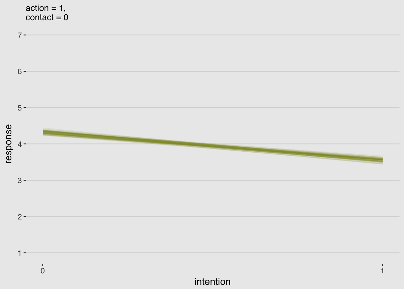
# Alternative to Figure 11.3.c
make_data_for_an_alternative_fiture(action = 0,
                                    contact = 1,
                                    max_iter = 100) %>%

  ggplot(aes(x = intention, y = mean_rating, group = iter)) +
  geom_line(alpha = 1/10, color = canva_pal("Green fields")(4)[1]) +
  scale_x_continuous(breaks = 0:1) +
  scale_y_continuous(breaks = 1:7) +
  coord_cartesian(ylim = 1:7) +
  labs(subtitle = "action = 0,\ncontact = 1",
       x = "intention",
       y = "response") +
  theme_hc() +
  theme(plot.background = element_rect(fill = "grey92"),
        legend.position = "none")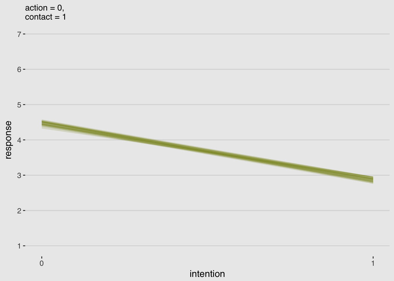
11.2. Zero-inflated outcomes
Very often, the things we can measure are not emissions from any pure process. Instead, they are mixtures of multiple processes. Whenever there are different causes for the same observation, then a mixture model may be useful. A mixture model uses more than one simple probability distribution to model a mixture of causes. In effect, these models use more than one likelihood for the same outcome variable.
Count variables are especially prone to needing a mixture treatment. The reason is that a count of zero can often arise more than one way. A “zero” means that nothing happened, and nothing can happen either because the rate of events is low or rather because the process that generates events failed to get started.
11.2.1. Example: Zero-inflated Poisson
A zero-inflated Poisson regression takes the form:
\[\begin{eqnarray} { y }_{ i } & \sim & \text{ZIPoisson}\left( p_i, \lambda_i \right) \\ \text{logit} \left( p_i \right) & = & \alpha_p + \beta_p x_i \\ \text{log} \left( \lambda_i \right) & = & \alpha_\lambda + \beta_\lambda x_i \end{eqnarray}\]
# define parameters
prob_drink <- 0.2  # 20% of days
rate_work  <- 1    # average 1 manuscript per day

# sample one year of production
N <- 365

# simulate days monks drink
set.seed(0.2)
drink <- rbinom(N, 1, prob_drink)

# simulate manuscripts completed
y <- (1 - drink)*rpois(N, rate_work)
d <-
tibble(Y = y) %>%
arrange(Y) %>%
mutate(zeros = c(rep("zeros_drink", times = sum(drink)),
rep("zeros_work", times = sum(y == 0 & drink == 0)),
rep("nope", times = N - sum(y == 0))))
ggplot(data = d, aes(x = Y)) +
geom_histogram(aes(fill = zeros),
binwidth = 1, color = "grey92") +
scale_fill_manual(values = c(canva_pal("Green fields")(4)[1],
canva_pal("Green fields")(4)[2],
canva_pal("Green fields")(4)[1])) +
xlab("Manuscripts completed") +
theme_hc() +
theme(plot.background = element_rect(fill = "grey92"),
legend.position = "none")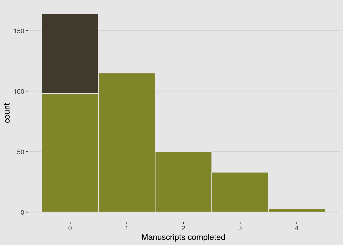
m11.4 <-
    brm(data = d, family = zero_inflated_poisson(),
        Y ~ 1,
        prior = c(set_prior("normal(0, 10)", class = "Intercept"),
                  # This is the brms default. See below.
                  set_prior("beta(1, 1)", class = "zi")),
        cores = 4)

print(m11.4)
## Family: zero_inflated_poisson
## Links: mu = log; zi = identity
## Formula: Y ~ 1
## Data: d (Number of observations: 365)
## Samples: 4 chains, each with iter = 2000; warmup = 1000; thin = 1;
## total post-warmup samples = 4000
##
## Population-Level Effects:
## Estimate Est.Error l-95% CI u-95% CI Eff.Sample Rhat
## Intercept 0.06 0.08 -0.11 0.22 931 1.00
##
## Family Specific Parameters:
## Estimate Est.Error l-95% CI u-95% CI Eff.Sample Rhat
## zi 0.15 0.06 0.04 0.26 927 1.00
##
## Samples were drawn using sampling(NUTS). For each parameter, Eff.Sample
## is a crude measure of effective sample size, and Rhat is the potential
## scale reduction factor on split chains (at convergence, Rhat = 1).zi in brms corresponds to the probability metric (p_i).
11.3. Over-dispersed outcomes
One symptom that something important has been omitted from a count model is over-dispersion. When the observed variance exceeds its theoretical value, after conditioning on all the predictor variables, this implies that some omitted variable is producing additional dispersion in the observed counts.
Ignoring over-dispersion can lead to all of the same problems as ignoring any predictor variable. Heterogeneity in counts can be a confound, hiding effects of interest or producing spurious inferences.
11.3.1. Beta-binomial
A beta-binomial model assumes that each binomial count observation has its own probability of a success. The model estimates the distribution of probabilities of success across cases, instead of a single probability of success. And predictor variables change the shape of this distribution, instead of directly determining the probability of each success.
pbar <- 0.5
theta <- 5

ggplot(data = tibble(x = seq(from = 0, to = 1, by = .01))) +
  geom_ribbon(aes(x = x,
                  ymin = 0,
                  ymax = rethinking::dbeta2(x, pbar, theta)),
              fill = canva_pal("Green fields")(4)[1]) +
  scale_x_continuous(breaks = c(0, .5, 1)) +
  scale_y_continuous(NULL, breaks = NULL) +
  labs(title = expression(paste("The ", beta, " distribution")),
       x = "probability space",
       y = "density") +
  theme_hc() +
  theme(plot.background = element_rect(fill = "grey92"))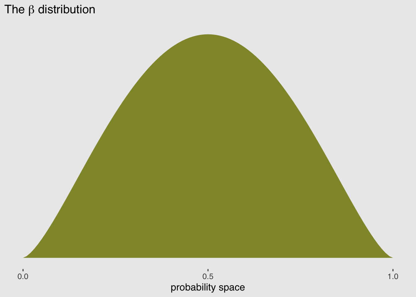
A beta-binomial model takes the form:
\[\begin{eqnarray} { A }_{ i } & \sim & \text{BetaBinomial}\left( n_i, p_i, \theta \right) \\ \text{logit} \left( p_i \right) & = & \alpha \\ \alpha & \sim & \text{Normal} \left( 0,10 \right) \\ \theta & \sim & \text{HalfCauchy} \left( 0,1 \right) \end{eqnarray}\]
To define your own custom probability family, follow this vignette.
library(rethinking)
data(UCBadmit)
d <- UCBadmit
rm(UCBadmit)
detach(package:rethinking, unload = T)
library(brms)
beta_binomial2 <-
custom_family(
"beta_binomial2", dpars = c("mu", "phi"),
links = c("logit", "log"), lb = c(NA, 0),
type = "int", vars = "trials[n]"
)
stan_funs <- "
real beta_binomial2_lpmf(int y, real mu, real phi, int T) {
return beta_binomial_lpmf(y | T, mu * phi, (1 - mu) * phi);
}
int beta_binomial2_rng(real mu, real phi, int T) {
return beta_binomial_rng(T, mu * phi, (1 - mu) * phi);
}
"The precision parameter can be rather fickle, so it’s better to use dexp instead of dcauchy and to specify a reasonable start value.
m11.5 <-
  brm(data = d,
      family = beta_binomial2,  # Here's our custom likelihood
      admit | trials(applications) ~ 1,
      prior = c(set_prior("normal(0, 2)", class = "Intercept"),
                set_prior("exponential(1)", class = "phi")),
      iter = 4000, warmup = 1000, cores = 2, chains = 2,
      stan_funs = stan_funs)

print(m11.5)
## Family: beta_binomial2
## Links: mu = logit; phi = identity
## Formula: admit | trials(applications) ~ 1
## Data: d (Number of observations: 12)
## Samples: 2 chains, each with iter = 4000; warmup = 1000; thin = 1;
## total post-warmup samples = 6000
##
## Population-Level Effects:
## Estimate Est.Error l-95% CI u-95% CI Eff.Sample Rhat
## Intercept -0.36 0.31 -0.97 0.26 4343 1.00
##
## Family Specific Parameters:
## Estimate Est.Error l-95% CI u-95% CI Eff.Sample Rhat
## phi 2.75 0.97 1.23 4.91 3844 1.00
##
## Samples were drawn using sampling(NUTS). For each parameter, Eff.Sample
## is a crude measure of effective sample size, and Rhat is the potential
## scale reduction factor on split chains (at convergence, Rhat = 1).post <- posterior_samples(m11.5)
tibble(x = 0:1) %>%
ggplot(aes(x = x)) +
stat_function(fun = rethinking::dbeta2,
args = list(prob = mean(invlogit(post[, 1])),
theta = mean(post[, 2])),
color = canva_pal("Green fields")(4)[4],
size = 1.5) +
mapply(function(prob, theta) {
stat_function(fun = rethinking::dbeta2,
args = list(prob = prob, theta = theta),
alpha = .2,
color = canva_pal("Green fields")(4)[4])
},
# Enter prob and theta, here
prob = invlogit(post[1:100, 1]),
theta = post[1:100, 2]) +
scale_y_continuous(NULL, breaks = NULL) +
coord_cartesian(ylim = 0:3) +
labs(x = "probability admit") +
theme_hc() +
theme(plot.background = element_rect(fill = "grey92"))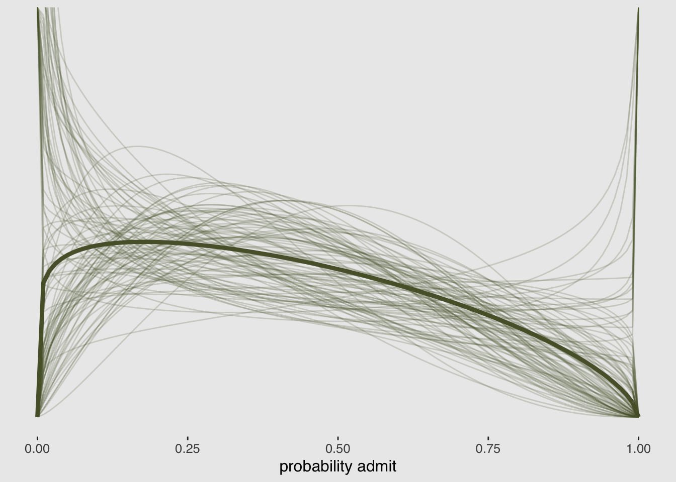
expose_functions(m11.5, vectorize = TRUE)

# Required to use `predict()`
log_lik_beta_binomial2 <-
  function(i, draws) {
    mu  <- draws$dpars$mu[, i]
    phi <- draws$dpars$phi
    N   <- draws$data$trials[i]
    y   <- draws$data$Y[i]
    beta_binomial2_lpmf(y, mu, phi, N)
  }

predict_beta_binomial2 <-
  function(i, draws, ...) {
    mu  <- draws$dpars$mu[, i]
    phi <- draws$dpars$phi
    N   <- draws$data$trials[i]
    beta_binomial2_rng(mu, phi, N)
  }

# Required to use `fitted()`
fitted_beta_binomial2 <-
  function(draws) {
    mu     <- draws$dpars$mu
    trials <- draws$data$trials
    trials <- matrix(trials, nrow = nrow(mu), ncol = ncol(mu), byrow = TRUE)
    mu * trials
  }
# The prediction intervals
predict(m11.5) %>%
as_tibble() %>%
rename(LL = Q2.5,
UL = Q97.5) %>%
select(LL:UL) %>%
# The fitted intervals
bind_cols(
fitted(m11.5) %>%
as_tibble()
) %>%
# The original data used to fit the model
bind_cols(m11.5$data) %>%
mutate(case = 1:12) %>%
ggplot(aes(x = case)) +
geom_linerange(aes(ymin = LL/applications,
ymax = UL/applications),
color = canva_pal("Green fields")(4)[1],
size = 2.5, alpha = 1/4) +
geom_pointrange(aes(ymin = Q2.5/applications,
ymax = Q97.5/applications,
y = Estimate/applications),
color = canva_pal("Green fields")(4)[4],
size = 1/2, shape = 1) +
geom_point(aes(y = admit/applications),
color = canva_pal("Green fields")(4)[2],
size = 2) +
scale_x_continuous(breaks = 1:12) +
scale_y_continuous(breaks = c(0, .5, 1)) +
coord_cartesian(ylim = 0:1) +
labs(subtitle = "Posterior validation check",
y = "Admittance probability") +
theme_hc() +
theme(plot.background = element_rect(fill = "grey92"),
axis.ticks.x = element_blank(),
legend.position = "none")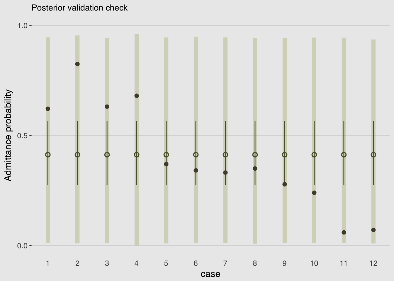
11.3.2. Negative-binomial or gamma-Poisson
A negative-binomial model, more usefully called a gamma-Poisson model, assumes that each Poisson count observation has its own rate.
11.3.3. Over-dispersion, entropy, and information criteria
Both the beta-binomial and gamma-Poisson models are maximum entropy for the same constraints as the regular binomial and Poisson. They just try to account for unobserved heterogeneity in probabilities and rates.
You should not use WAIC with these models, however, unless you are very sure of what you are doing. The reason is that while ordinary binomial and Poisson models can be aggregated and disaggregated across rows in the data, without changing any causal assumptions, the same is not true of beta-binomial and gamma-Poisson models. The reason is that a betabinomial or gamma-Poisson likelihood applies an unobserved parameter to each row in the data. When we then go to calculate log-likelihoods, how the data are structured will determine how the beta-distributed or gamma-distributed variation enters the model.
What to do? In most cases, you’ll want to fall back on DIC, which doesn’t force a decomposition of the log-likelihood. Consider also using multilevel models.
References
McElreath, R. (2016). Statistical rethinking: A Bayesian course with examples in R and Stan. Chapman & Hall/CRC Press.
Kurz, A. S. (2018, March 9). brms, ggplot2 and tidyverse code, by chapter. Retrieved from https://goo.gl/JbvNTj