Multilevel models remember features of each cluster in the data as they learn about all of the clusters. Depending upon the variation among clusters, which is learned from the data as well, the model pools information across clusters. This pooling tends to improve estimates about each cluster. This improved estimation leads to several, more pragmatic sounding, benefits of the multilevel approach.
- Improved estimates for repeat sampling. When more than one observation arises from the same individual, location, or time, then traditional, single-level models either maximally underfit or overfit the data.
- Improved estimates for imbalance in sampling. When some individuals, locations, or times are sampled more than others, multilevel models automatically cope with differing uncertainty across these clusters. This prevents over-sampled clusters from unfairly dominating inference.
- Estimates of variation. If our research questions include variation among individuals or other groups within the data, then multilevel models are a big help, because they model variation explicitly.
- Avoid averaging, retain variation. Frequently, scholars pre-average some data to construct variables. This can be dangerous, because averaging removes variation, and there are also typically several different ways to perform the averaging. Averaging therefore both manufactures false confidence and introduces arbitrary data transformations. Multilevel models allow us to preserve the uncertainty and avoid data transformations.
There are costs of the multilevel approach. The first is that we have to make some new assumptions. We have to define the distributions from which the characteristics of the clusters arise. Luckily, conservative maximum entropy distributions do an excellent job in this context. Second, there are new estimation challenges that come with the full multilevel approach. These challenges lead us headfirst into MCMC estimation. Third, multilevel models can be hard to understand, because they make predictions at different levels of the data. In many cases, we are interested in only one or a few of those levels, and as a consequence, model comparison using metrics like DIC and WAIC becomes more subtle. The basic logic remains unchanged, but now we have to make more decisions about which parameters in the model we wish to focus on.
The most common synonyms for “multilevel” are hierarchical and mixed effects. The type of parameters that appear in multilevel models are most commonly known as random effects.
12.1. Example: Multilevel tadpoles
library(rethinking)
data(reedfrogs)
d <- reedfrogs
rm(reedfrogs)
detach(package:rethinking, unload = T)
library(brms)
library(tidyverse)
d %>%
glimpse()## Observations: 48
## Variables: 5
## $ density <int> 10, 10, 10, 10, 10, 10, 10, 10, 10, 10, 10, 10, 10, 1...
## $ pred <fct> no, no, no, no, no, no, no, no, pred, pred, pred, pre...
## $ size <fct> big, big, big, big, small, small, small, small, big, ...
## $ surv <int> 9, 10, 7, 10, 9, 9, 10, 9, 4, 9, 7, 6, 7, 5, 9, 9, 24...
## $ propsurv <dbl> 0.90, 1.00, 0.70, 1.00, 0.90, 0.90, 1.00, 0.90, 0.40,...d <-
d %>%
mutate(tank = 1:nrow(d))Varying intercepts are the simplest kind of varying effects.
\[\begin{eqnarray} { s }_{ i } & \sim & \text{Binomial}\left( n_i, p_i \right) & \text{<- likelihood } \\ \text{logit} \left( p_i \right) & = & \alpha_{\text{TANK}[i]} & \text{<- log-odds for tank on row }i\\ \alpha_{\text{TANK}[i]} & \sim & \text{Normal} \left( \alpha,\sigma \right) & \text{<- varying intercepts prior } \\ \alpha & \sim & \text{Normal} \left( 0,1 \right) & \text{<- prior of average tank } \\ \sigma & \sim & \text{HalfCauchy} \left( 0,1 \right) & \text{<- prior of standard deviation of tanks } \end{eqnarray}\]
These two parameters, \(\alpha\) and \(\sigma\), are often referred to as hyperparameters. They are parameters for parameters. And their priors are often called hyperpriors. In principle, there is no limit to how many “hyper” levels you can install in a model. For example, different populations of tanks could be embedded within different regions of habitat. But in practice there are limits, both because of computation and our ability to understand the model.
Why Gaussian tanks? In the multilevel tadpole model, the population of tanks is assumed to be Gaussian. Why? The least satisfying answer is “convention.” The Gaussian assumption is extremely common. A more satisfying answer is “pragmatism.” The Gaussian assumption is easy to work with, and it generalizes easily to more than one dimension. This generalization will be important for handling varying slopes in the next chapter. But my preferred answer is instead “entropy.” If all we are willing to say about a distribution is the mean and variance, then the Gaussian is the most conservative assumption. There is no rule requiring the Gaussian distribution of varying effects, though. So if you have a good reason to use another distribution, then do so.
# unpooled model
m12.1 <-
    brm(data = d, family = binomial,
        surv | trials(density) ~ 0 + factor(tank),
        prior = c(set_prior("normal(0, 5)", class = "b")),
        chains = 4, iter = 2000, warmup = 500, cores = 4)
# pooled model
m12.2 <-
brm(data = d, family = binomial,
surv | trials(density) ~ 1 + (1 | tank),
prior = c(set_prior("normal(0, 1)", class = "Intercept"),
set_prior("cauchy(0, 1)", class = "sd")),
chains = 4, iter = 4000, warmup = 1000, cores = 4)
print(m12.2)## Family: binomial
## Links: mu = logit
## Formula: surv | trials(density) ~ 1 + (1 | tank)
## Data: d (Number of observations: 48)
## Samples: 4 chains, each with iter = 4000; warmup = 1000; thin = 1;
## total post-warmup samples = 12000
##
## Group-Level Effects:
## ~tank (Number of levels: 48)
## Estimate Est.Error l-95% CI u-95% CI Eff.Sample Rhat
## sd(Intercept) 1.62 0.21 1.25 2.09 3296 1.00
##
## Population-Level Effects:
## Estimate Est.Error l-95% CI u-95% CI Eff.Sample Rhat
## Intercept 1.30 0.25 0.81 1.81 2473 1.00
##
## Samples were drawn using sampling(NUTS). For each parameter, Eff.Sample
## is a crude measure of effective sample size, and Rhat is the potential
## scale reduction factor on split chains (at convergence, Rhat = 1).#kf <- kfold(m12.1, m12.2,
# K = 10)
#kfThe \(K\)-fold cross-validation difference of 59, with a standard error around 9, suggests that model m12.2 is the clear favorite relative to m12.1.
post <- posterior_samples(m12.2)

invlogit <- function(x){1/(1+exp(-x))}

postMdn <-
  coef(m12.2, robust = T) %>% data.frame() %>%
  add_column(tank = d$tank,
             density = d$density,
             propsurv = d$propsurv) %>%
  mutate(postMdn = invlogit(tank.Estimate.Intercept))

library(ggthemes)

postMdn %>%
  ggplot(aes(x = tank, y = postMdn)) +
  theme_fivethirtyeight() +
  geom_hline(yintercept = invlogit(median(post$b_Intercept)), linetype = 2, size = 1/4) +
  geom_vline(xintercept = c(16.5, 32.5), size = 1/4) +
  geom_point(shape = 1) +
  geom_point(aes(y = propsurv), color = "orange2") +
  coord_cartesian(ylim = c(0, 1)) +
  scale_x_continuous(breaks = c(1, 16, 32, 48)) +
  labs(title = "Proportion of survivors in each tank",
       subtitle = "The empirical proportions are in orange while the\nmodel-implied proportions are the black circles.\nThe dashed line is the model-implied average survival proportion.") +
  annotate("text", x = c(8, 16 + 8, 32 + 8), y = 0,
           label = c("small tanks", "medium tanks", "large tanks")) +
  theme(panel.grid = element_blank())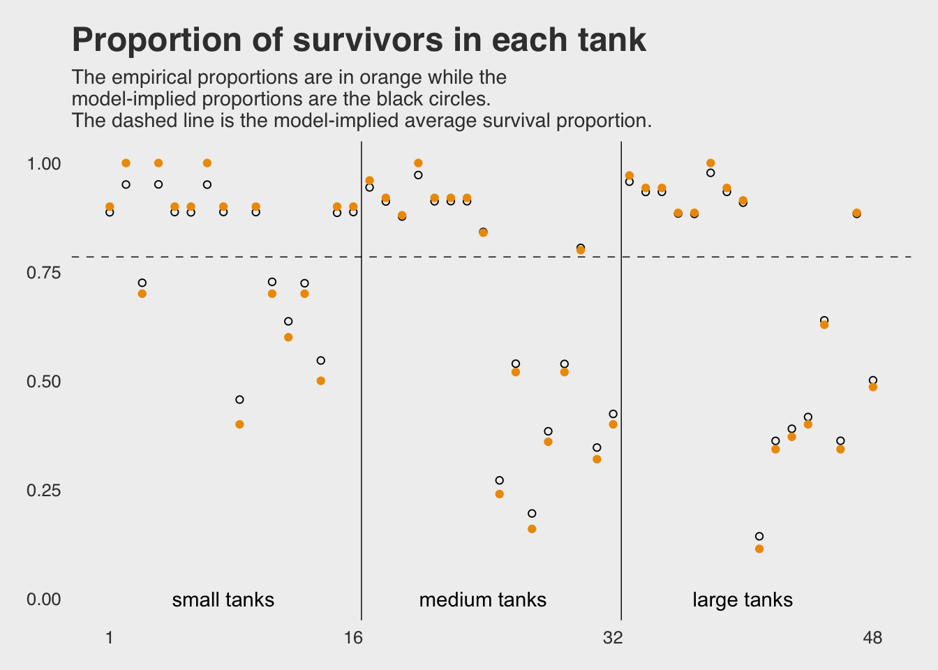
The plot above shows pooling information across clusters (tanks) to improve estimates. What pooling means here is that each tank provides information that can be used to improve the estimates for all of the other tanks. Each tank helps in this way, because we made an assumption about how the varying log-odds in each tank related to all of the others. We assumed a distribution, the normal distribution in this case. Once we have a distributional assumption, we can use Bayes’ theorem to optimally (in the small world only) share information among the clusters.
Remember that “sampling” from a posterior distribution is not a simulation of empirical sampling. It’s just a convenient way to characterize and work with the uncertainty in the distribution.
tibble(x = c(-3, 4)) %>%

  ggplot(aes(x = x)) +
  theme_fivethirtyeight() +
  mapply(function(mean, sd) {
    stat_function(fun = dnorm,
                  args = list(mean = mean, sd = sd),
                  alpha = .2,
                  color = "orange2")
  },
  # Enter means and standard deviations here
  mean = post[1:100, 1],
  sd = post[1:100, 2]
  ) +
  labs(title = "Survival in log-odds") +
  scale_y_continuous(NULL, breaks = NULL)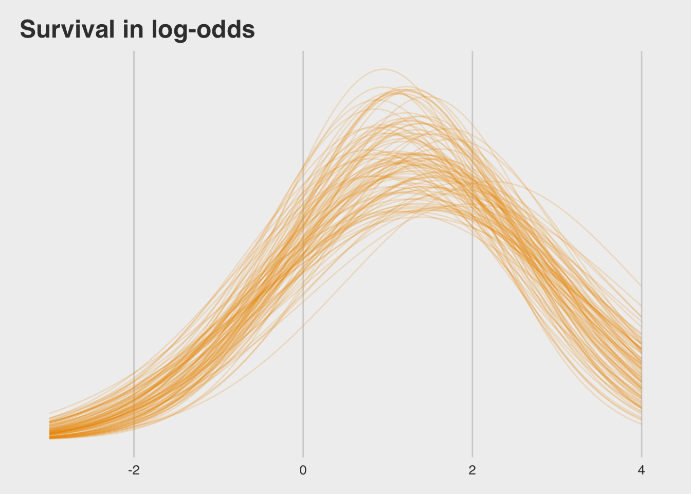
ggplot(data = post,
       aes(x = invlogit(rnorm(nrow(post), mean = post[, 1], sd = post[, 2])))) +
  theme_fivethirtyeight() +
  geom_density(size = 0, fill = "orange2") +
  labs(title = "Probability of survival") +
  scale_y_continuous(NULL, breaks = NULL)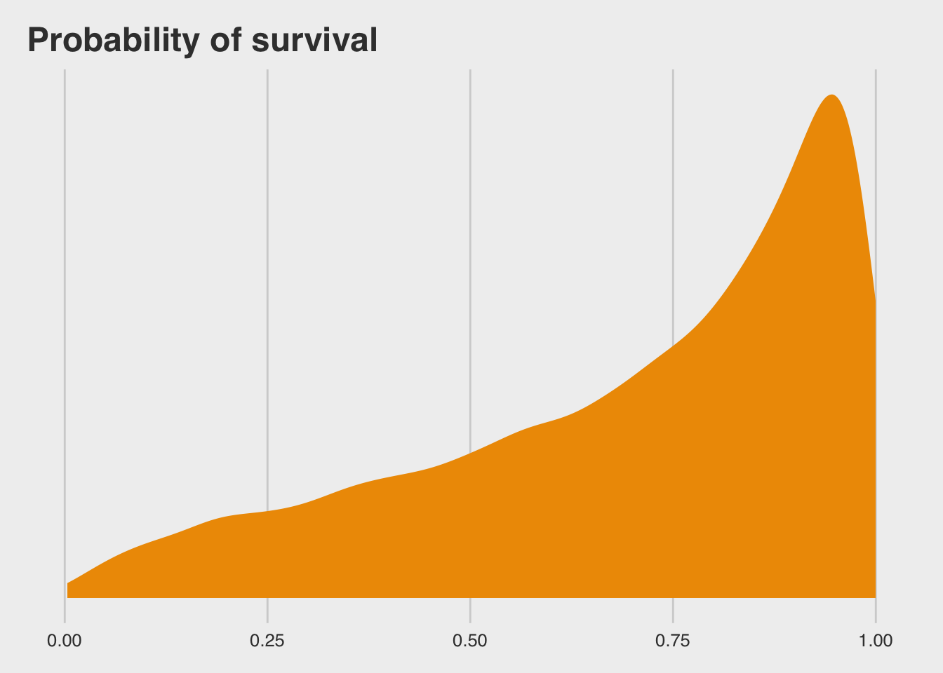
Instead of using half-Cauchy priors for the variance components, you can use exponential priors.
m12.2.e <-
  brm(data = d, family = binomial,
      surv | trials(density) ~ 1 + (1 | tank),
      prior = c(set_prior("normal(0, 1)", class = "Intercept"),
                set_prior("exponential(1)", class = "sd")),
      chains = 4, iter = 2000, warmup = 500, cores = 4)
ggplot(data = tibble(x = seq(from = 0, to = 4, by = .01)),
aes(x = x)) +
theme_fivethirtyeight()+
geom_ribbon(aes(ymin = 0, ymax = dexp(x, rate = 1)), # the prior
fill = "orange2", alpha = 1/3) +
geom_density(data = posterior_samples(m12.2.e), # the posterior
aes(x = sd_tank__Intercept),
size = 0, fill = "orange2") +
geom_vline(xintercept = posterior_samples(m12.2.e)[, 2] %>% median(),
color = "blue", linetype = 2) +
scale_y_continuous(NULL, breaks = NULL) +
coord_cartesian(xlim = c(0, 3.5)) +
labs(title = "Bonus prior/posterior plot\n for `sd_tank__Intercept`",
subtitle = "The prior is the semitransparent ramp in the\nbackground. The posterior is the solid orange\nmound. The dashed line is the posterior median.")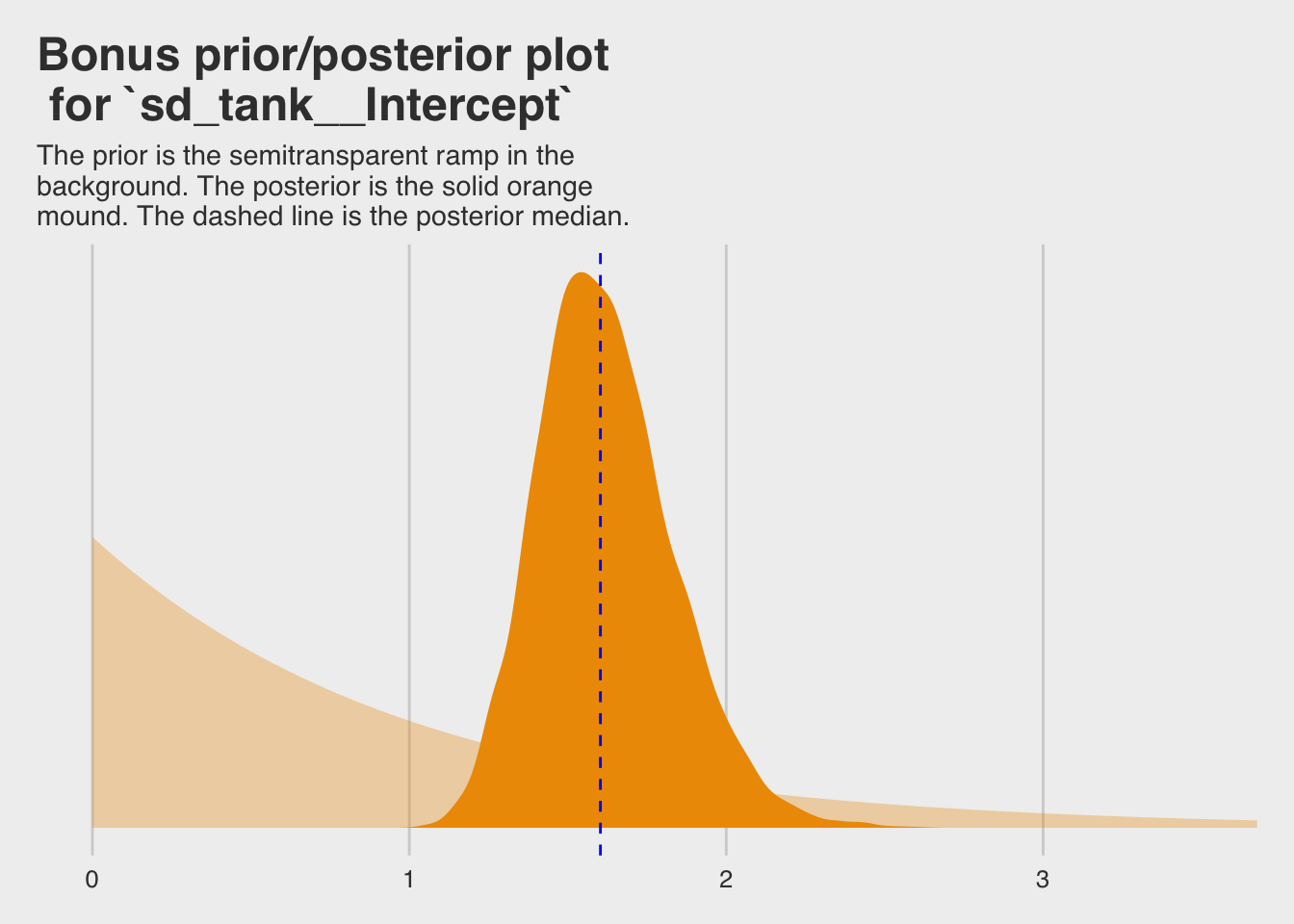
12.2. Varying effects and the underfitting/overfitting trade-off
Varying intercepts are just regularized estimates, but adaptively regularized by estimating how diverse the clusters are while estimating the features of each cluster.
A major benefit of using varying effects estimates, instead of the empirical raw estimates, is that they provide more accurate estimates of the individual cluster (tank) intercepts. On average, the varying effects actually provide a better estimate of the individual tank (cluster) means. The reason that the varying intercepts provide better estimates is that they do a better job of trading off underfitting and overfitting.
There are three ways of modelling:
- Complete pooling. This means we assume that the population of ponds is invariant, the same as estimating a common intercept for all ponds. However, your estimate is unlikely to exactly match the intercept of any particular pond. As a result, the total sample intercept underfits the data. This sort of model is equivalent to assuming that the variation among ponds is zero.
- No pooling. This means we assume that each pond tells us nothing about any other pond. This is the model with amnesia. As a consequence, the error of these estimates is high, and they are rather overfit to the data. Standard errors for each intercept can be very large, and in extreme cases, even infinite.
- Partial pooling. This means using an adaptive regularizing prior. This produces estimates for each cluster that are less underfit than the grand mean and less overfit than the no-pooling estimates.
The model
\[\begin{eqnarray} { s }_{ i } & \sim & \text{Binomial}\left( n_i, p_i \right) \\ \text{logit} \left( p_i \right) & = & \alpha_{\text{POND}[i]} \\ \alpha_{\text{POND}[i]} & \sim & \text{Normal} \left( \alpha,\sigma \right) \\ \alpha & \sim & \text{Normal} \left( 0,1 \right) \\ \sigma & \sim & \text{HalfCauchy} \left( 0,1 \right) \end{eqnarray}\]
12.2.2. Assign values to the parameters
a      <- 1.4
sigma  <- 1.5
nponds <- 60
ni     <- rep(c(5, 10, 25, 35), each = 15) %>% as.integer()

set.seed(10579595) # To make results reproducible
dsim <-
  tibble(pond = 1:nponds,
         ni = ni,
         true_a = rnorm(nponds, mean = a, sd = sigma))
12.2.3. Simulate survivors
set.seed(10579595) # To make results reproducible
dsim <-
  dsim %>%
  mutate(si = rbinom(nponds, prob = invlogit(true_a), size = ni)) %>%
  mutate(p_nopool = si/ni)

dsim %>%
  glimpse()
## Observations: 60
## Variables: 5
## $ pond <int> 1, 2, 3, 4, 5, 6, 7, 8, 9, 10, 11, 12, 13, 14, 15, 16...
## $ ni <int> 5, 5, 5, 5, 5, 5, 5, 5, 5, 5, 5, 5, 5, 5, 5, 10, 10, ...
## $ true_a <dbl> 3.1085100, 3.6798855, 2.6097976, 4.2842340, 3.2304515...
## $ si <int> 4, 5, 4, 5, 5, 4, 4, 2, 4, 2, 5, 4, 2, 4, 4, 10, 7, 1...
## $ p_nopool <dbl> 0.8, 1.0, 0.8, 1.0, 1.0, 0.8, 0.8, 0.4, 0.8, 0.4, 1.0...12.2.5. Compute the partial-pooling estimates
m12.3 <-
  brm(data = dsim, family = binomial,
      si | trials(ni) ~ 1 + (1 | pond),
      prior = c(set_prior("normal(0, 1)", class = "Intercept"),
                set_prior("cauchy(0, 1)", class = "sd")),
      chains = 1, iter = 10000, warmup = 1000, cores = 1)
##
## SAMPLING FOR MODEL 'binomial brms-model' NOW (CHAIN 1).
##
## Gradient evaluation took 5.5e-05 seconds
## 1000 transitions using 10 leapfrog steps per transition would take 0.55 seconds.
## Adjust your expectations accordingly!
##
##
## Iteration: 1 / 10000 [ 0%] (Warmup)
## Iteration: 1000 / 10000 [ 10%] (Warmup)
## Iteration: 1001 / 10000 [ 10%] (Sampling)
## Iteration: 2000 / 10000 [ 20%] (Sampling)
## Iteration: 3000 / 10000 [ 30%] (Sampling)
## Iteration: 4000 / 10000 [ 40%] (Sampling)
## Iteration: 5000 / 10000 [ 50%] (Sampling)
## Iteration: 6000 / 10000 [ 60%] (Sampling)
## Iteration: 7000 / 10000 [ 70%] (Sampling)
## Iteration: 8000 / 10000 [ 80%] (Sampling)
## Iteration: 9000 / 10000 [ 90%] (Sampling)
## Iteration: 10000 / 10000 [100%] (Sampling)
##
## Elapsed Time: 0.780968 seconds (Warm-up)
## 5.34393 seconds (Sampling)
## 6.1249 seconds (Total)print(m12.3)## Family: binomial
## Links: mu = logit
## Formula: si | trials(ni) ~ 1 + (1 | pond)
## Data: dsim (Number of observations: 60)
## Samples: 1 chains, each with iter = 10000; warmup = 1000; thin = 1;
## total post-warmup samples = 9000
##
## Group-Level Effects:
## ~pond (Number of levels: 60)
## Estimate Est.Error l-95% CI u-95% CI Eff.Sample Rhat
## sd(Intercept) 1.34 0.19 1.02 1.76 2954 1.00
##
## Population-Level Effects:
## Estimate Est.Error l-95% CI u-95% CI Eff.Sample Rhat
## Intercept 1.29 0.20 0.90 1.70 2573 1.00
##
## Samples were drawn using sampling(NUTS). For each parameter, Eff.Sample
## is a crude measure of effective sample size, and Rhat is the potential
## scale reduction factor on split chains (at convergence, Rhat = 1).coef(m12.3)$pond %>%
round(digits = 2)## , , Intercept
##
## Estimate Est.Error Q2.5 Q97.5
## 1 1.46 0.87 -0.11 3.27
## 2 2.36 1.03 0.55 4.58
## 3 1.46 0.89 -0.17 3.36
## 4 2.36 1.05 0.50 4.59
## 5 2.36 1.06 0.50 4.69
## 6 1.46 0.89 -0.18 3.33
## 7 1.46 0.89 -0.17 3.33
## 8 0.14 0.80 -1.44 1.71
## 9 1.46 0.90 -0.17 3.38
## 10 0.14 0.79 -1.42 1.70
## 11 2.35 1.05 0.51 4.58
## 12 1.46 0.89 -0.19 3.32
## 13 0.13 0.78 -1.44 1.72
## 14 1.46 0.88 -0.15 3.33
## 15 1.47 0.89 -0.14 3.34
## 16 2.75 0.96 1.13 4.82
## 17 1.01 0.65 -0.21 2.38
## 18 2.74 0.96 1.11 4.85
## 19 2.01 0.81 0.58 3.74
## 20 1.46 0.72 0.15 2.92
## 21 0.26 0.58 -0.87 1.41
## 22 1.01 0.65 -0.22 2.35
## 23 0.62 0.61 -0.55 1.85
## 24 1.01 0.65 -0.18 2.31
## 25 2.75 0.98 1.10 4.88
## 26 2.02 0.80 0.58 3.73
## 27 2.01 0.80 0.59 3.75
## 28 2.75 0.96 1.07 4.85
## 29 0.26 0.59 -0.91 1.44
## 30 2.75 0.97 1.10 4.90
## 31 0.50 0.40 -0.27 1.32
## 32 -0.27 0.39 -1.04 0.49
## 33 1.96 0.55 0.98 3.14
## 34 2.73 0.72 1.49 4.32
## 35 2.30 0.63 1.18 3.65
## 36 0.50 0.41 -0.28 1.32
## 37 3.30 0.86 1.83 5.17
## 38 1.43 0.48 0.55 2.43
## 39 2.30 0.62 1.20 3.63
## 40 0.67 0.41 -0.13 1.48
## 41 -1.12 0.45 -2.04 -0.29
## 42 0.34 0.40 -0.43 1.14
## 43 0.50 0.40 -0.28 1.30
## 44 0.35 0.40 -0.43 1.13
## 45 3.32 0.87 1.86 5.25
## 46 0.98 0.37 0.27 1.73
## 47 3.54 0.85 2.11 5.41
## 48 -0.20 0.34 -0.86 0.46
## 49 2.27 0.53 1.33 3.36
## 50 0.97 0.37 0.28 1.71
## 51 1.26 0.39 0.53 2.07
## 52 -0.19 0.33 -0.86 0.44
## 53 0.25 0.34 -0.41 0.91
## 54 2.02 0.49 1.13 3.06
## 55 -0.78 0.36 -1.50 -0.10
## 56 1.42 0.41 0.64 2.26
## 57 -1.19 0.40 -2.00 -0.44
## 58 -0.53 0.34 -1.22 0.12
## 59 1.60 0.43 0.81 2.49
## 60 2.61 0.60 1.53 3.89p_partpool <-
coef(m12.3) %>%
data.frame() %>% # as_tibble() didn't work well, for this.
select(pond.Estimate.Intercept) %>%
mutate(pond.Estimate.Intercept = invlogit(pond.Estimate.Intercept)) %>%
pull()
dsim <-
dsim %>%
mutate(p_true = invlogit(true_a)) %>%
mutate(nopool_error = abs(p_nopool - p_true)) %>%
mutate(partpool_error = abs(p_partpool - p_true))
dsim %>%
glimpse()## Observations: 60
## Variables: 8
## $ pond <int> 1, 2, 3, 4, 5, 6, 7, 8, 9, 10, 11, 12, 13, 14, ...
## $ ni <int> 5, 5, 5, 5, 5, 5, 5, 5, 5, 5, 5, 5, 5, 5, 5, 10...
## $ true_a <dbl> 3.1085100, 3.6798855, 2.6097976, 4.2842340, 3.2...
## $ si <int> 4, 5, 4, 5, 5, 4, 4, 2, 4, 2, 5, 4, 2, 4, 4, 10...
## $ p_nopool <dbl> 0.8, 1.0, 0.8, 1.0, 1.0, 0.8, 0.8, 0.4, 0.8, 0....
## $ p_true <dbl> 0.9572424, 0.9753948, 0.9314895, 0.9864032, 0.9...
## $ nopool_error <dbl> 0.15724241, 0.02460518, 0.13148948, 0.01359676,...
## $ partpool_error <dbl> 0.145830683, 0.061708916, 0.119849691, 0.072617...dfline <-
dsim %>%
select(ni, nopool_error:partpool_error) %>%
gather(key, value, -ni) %>%
group_by(key, ni) %>%
summarise(mean_error = mean(value)) %>%
mutate(x = c(1, 16, 31, 46),
xend = c(15, 30, 45, 60))
ggplot(data = dsim, aes(x = pond)) +
theme_fivethirtyeight() +
geom_vline(xintercept = c(15.5, 30.5, 45.4),
color = "white", size = 2/3) +
geom_point(aes(y = nopool_error), color = "orange2") +
geom_point(aes(y = partpool_error), shape = 1) +
geom_segment(data = dfline,
aes(x = x, xend = xend,
y = mean_error, yend = mean_error),
color = rep(c("orange2", "black"), each = 4),
linetype = rep(1:2, each = 4)) +
labs(y = "absolute error",
title = "Estimate error by model type",
subtitle = "The horizontal axis displays pond number. The vertical\naxis measures the absolute error in the predicted proportion\nof survivors, compared to the true value used in the simulation.\nThe higher the point, the worse the estimate. No-pooling shown\nin orange. Partial pooling shown in black. The orange and\ndashed black lines show the average error for each kind of\nestimate, across each initial density of tadpoles (pond size).\nSmaller ponds produce more error, but the partial pooling\nestimates are better on average, especially in smaller ponds.") +
scale_x_continuous(breaks = c(1, 10, 20, 30, 40, 50, 60)) +
annotate("text", x = c(15 - 7.5, 30 - 7.5, 45 - 7.5, 60 - 7.5), y = .45,
label = c("tiny (5)", "small (10)", "medium (25)", "large (35)")) +
theme(panel.grid = element_blank())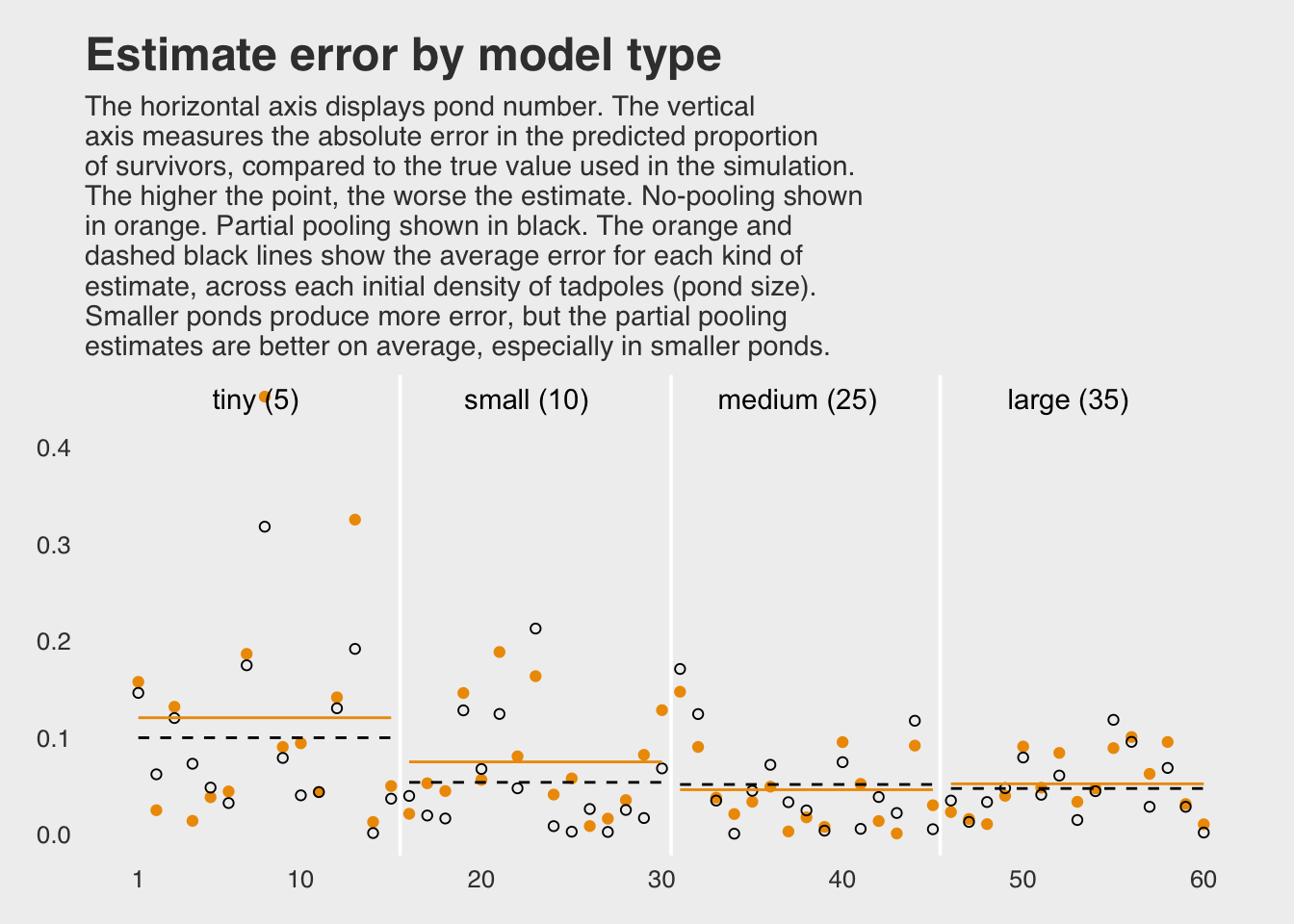
dsim %>%
  select(ni, nopool_error:partpool_error) %>%
  gather(key, value, -ni) %>%
  group_by(key) %>%
  summarise(mean_error   = mean(value) %>% round(digits = 3),
            median_error = median(value) %>% round(digits = 3))
## # A tibble: 2 x 3
## key mean_error median_error
## <chr> <dbl> <dbl>
## 1 nopool_error 0.073 0.048
## 2 partpool_error 0.063 0.04212.3. More than one type of cluster
References
McElreath, R. (2016). Statistical rethinking: A Bayesian course with examples in R and Stan. Chapman & Hall/CRC Press.
Kurz, A. S. (2018, March 9). brms, ggplot2 and tidyverse code, by chapter. Retrieved from https://goo.gl/JbvNTj