Linear regression is a family of simple statistical golems that attempt to learn about the mean and variance of some measurement, using an additive combination of other measurements. Linear regression can usefully describe a very large variety of natural phenomena, and it is a descriptive model that corresponds to many different process models.
4.1. Why normal distributions are normal
4.1.1. Normal by addition
Any process that adds together random values from the same distribution converges to a normal.
library(tidyverse)

set.seed(1000)
pos <-
  replicate(100, runif(16, -1, 1)) %>%        # Here is the simulation
  as_tibble() %>%                             # For data manipulation, we will make this a tibble
  rbind(0, .) %>%                             # Here we add a row of zeros above the simulation results
  mutate(step = 0:16) %>%                     # This adds our step index
  gather(key, value, -step) %>%               # Here we convert the data to the long format
  mutate(person = rep(1:100, each = 17)) %>%  # This adds a person id index
  # The next two lines allows us to make culmulative sums within each person
  group_by(person) %>%
  mutate(position = cumsum(value)) %>%
  ungroup()  # Ungrouping allows for further data manipulation

pos %>%
  filter(step == 16) %>%
  ggplot(aes(x = position)) +
  geom_density(color = "dodgerblue1") + #geom_line(stat = "density", color = "dodgerblue1") +
  coord_cartesian(xlim = -6:6) +
  labs(title = "16 steps")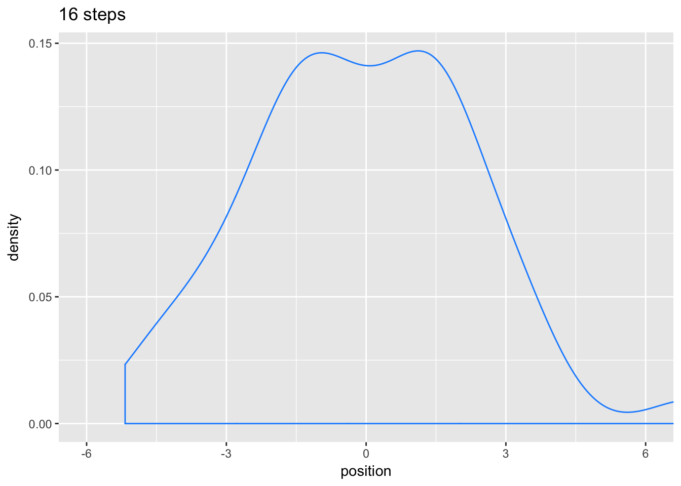
4.1.2. Normal by multiplication
Small effects that multiply together are approximately additive, and so they also tend to stabilize on Gaussian distributions.
set.seed(.1)
growth <-
  replicate(10000, prod(1 + runif(12, 0, 0.1))) %>%
  as_tibble()

ggplot(data = growth, aes(x = value)) +
  geom_density(color = "dodgerblue1")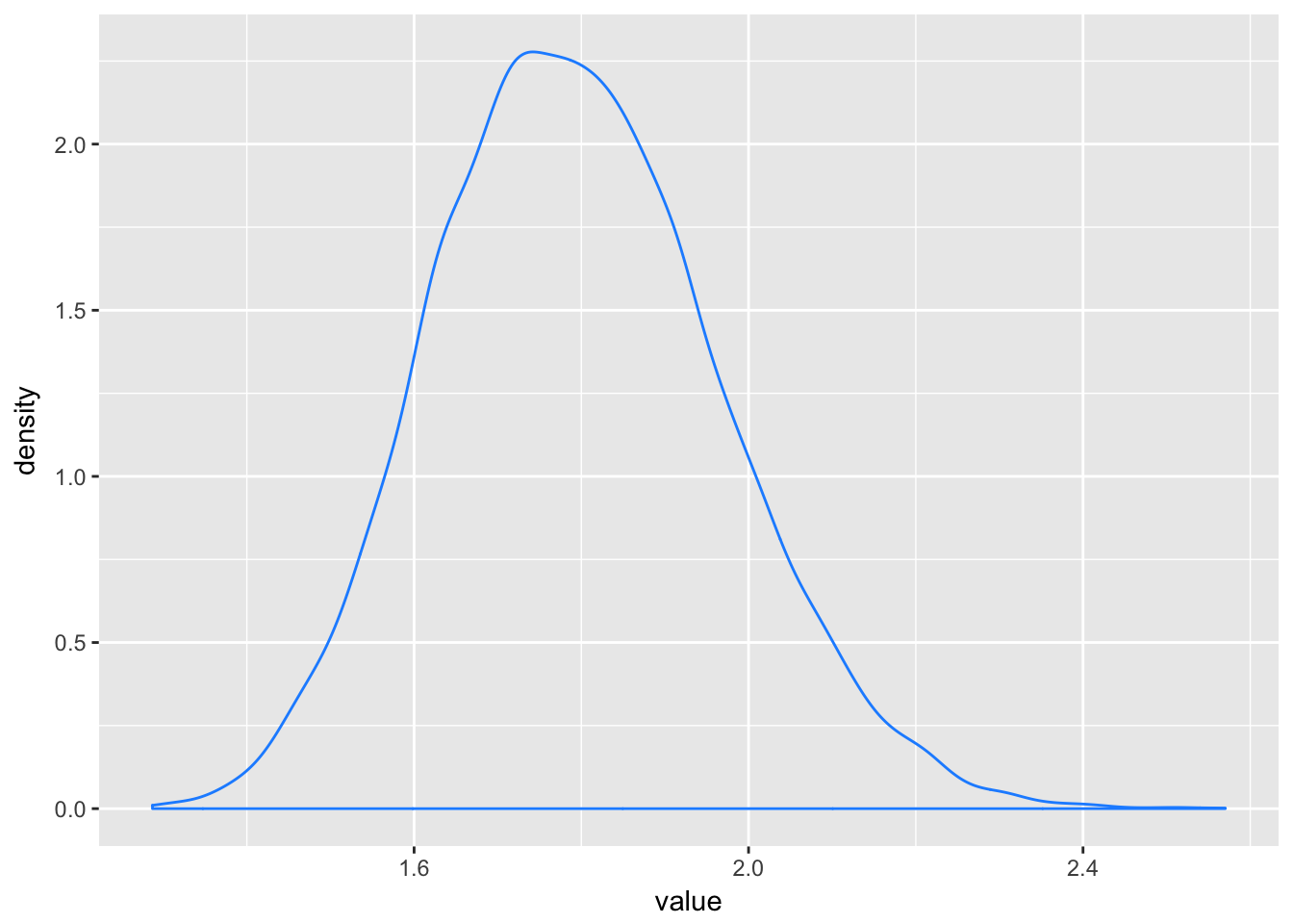
4.1.3. Normal by log-multiplication
Large deviates that are multiplied together do not produce Gaussian distributions, but they do tend to produce Gaussian distributions on the log scale.
set.seed(12)
replicate(10000, log(prod(1 + runif(12,0,0.5)))) %>%
    as_tibble() %>%
    ggplot(aes(x = value)) +
    geom_density(color = "dodgerblue1")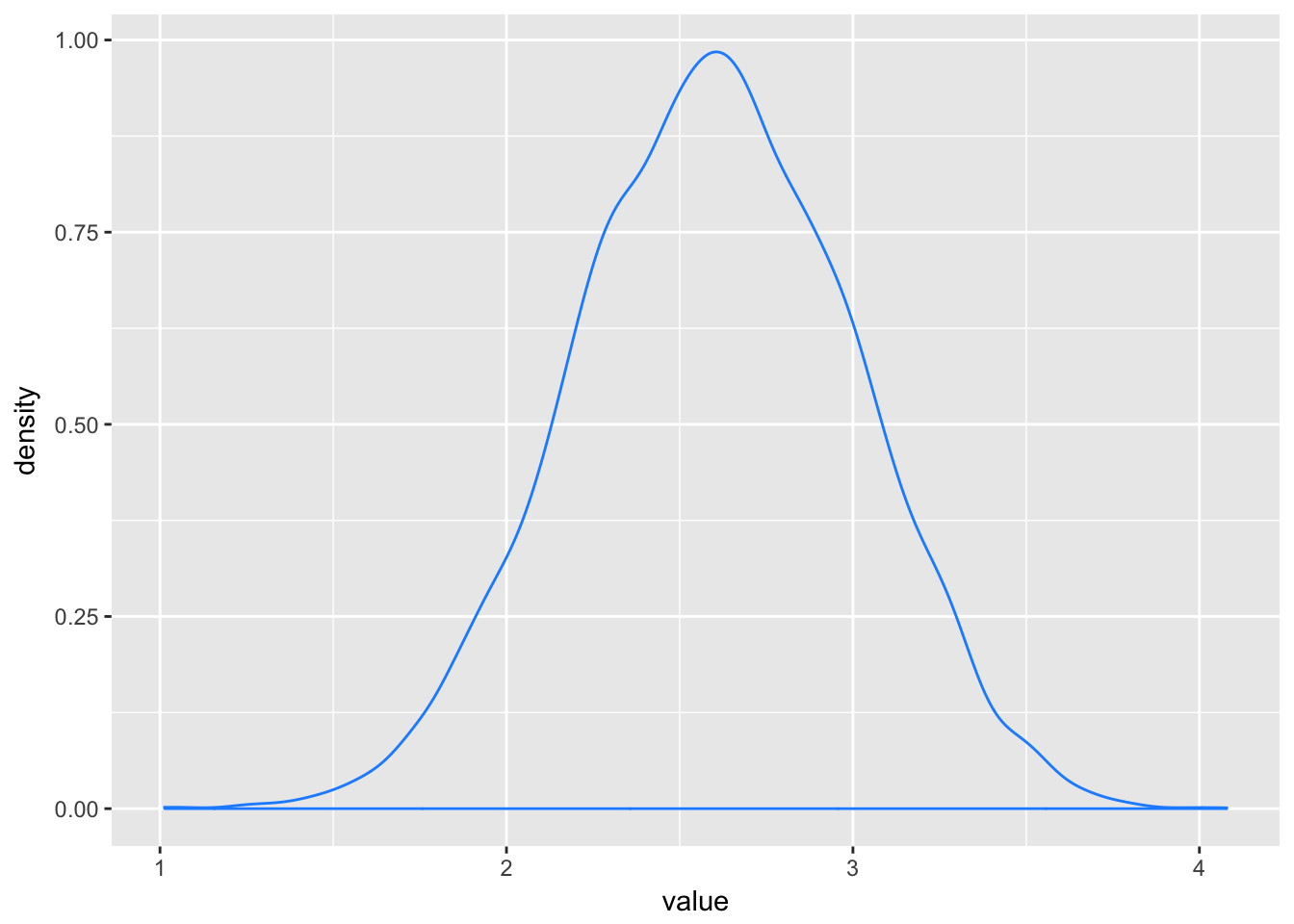
4.1.4. Using Gaussian distributions
4.1.4.1. Ontological justification
The world is full of Gaussian distributions, approximately. As a mathematical idealization, we’re never going to experience a perfect Gaussian distribution. But it is a widespread pattern, appearing again and again at different scales and in different domains. Measurement errors, variations in growth, and the velocities of molecules all tend towards Gaussian distributions. These processes do this because at their heart, these processes add together fluctuations. And repeatedly adding finite fluctuations results in a distribution of sums that have shed all information about the underlying process, aside from mean and spread. One consequence of this is that statistical models based on Gaussian distributions cannot reliably identify micro-process. But it also means that these models can do useful work, even when they cannot identify process.
4.1.4.2 Epistemological justification
The Gaussian distribution is the most natural expression of our state of ignorance, because if all we are willing to assume is that a measure has finite variance, the Gaussian distribution is the shape that can be realized in the largest number of ways and does not introduce any new assumptions. It is the least surprising and least informative assumption to make.
4.3. A Gaussian model of height
4.3.1. The data
# Load data from the rethinking package
library(rethinking)
data(Howell1)
d <- Howell1

# Have a look at the data
d %>% glimpse()
## Observations: 544
## Variables: 4
## $ height <dbl> 151.7650, 139.7000, 136.5250, 156.8450, 145.4150, 163.8...
## $ weight <dbl> 47.82561, 36.48581, 31.86484, 53.04191, 41.27687, 62.99...
## $ age <dbl> 63.0, 63.0, 65.0, 41.0, 51.0, 35.0, 32.0, 27.0, 19.0, 5...
## $ male <int> 1, 0, 0, 1, 0, 1, 0, 1, 0, 1, 0, 1, 0, 0, 0, 1, 1, 0, 1...# Filter heights of adults in the sample. The reason to filter out non-adults is that height is strongly correlated with age, before adulthood.
d2 <- d %>% filter(age >= 18) %>% glimpse()## Observations: 352
## Variables: 4
## $ height <dbl> 151.7650, 139.7000, 136.5250, 156.8450, 145.4150, 163.8...
## $ weight <dbl> 47.82561, 36.48581, 31.86484, 53.04191, 41.27687, 62.99...
## $ age <dbl> 63.0, 63.0, 65.0, 41.0, 51.0, 35.0, 32.0, 27.0, 19.0, 5...
## $ male <int> 1, 0, 0, 1, 0, 1, 0, 1, 0, 1, 0, 1, 0, 0, 0, 1, 1, 0, 1...4.3.2. The model
d2 %>%
    ggplot(aes(x = height)) +
    geom_density()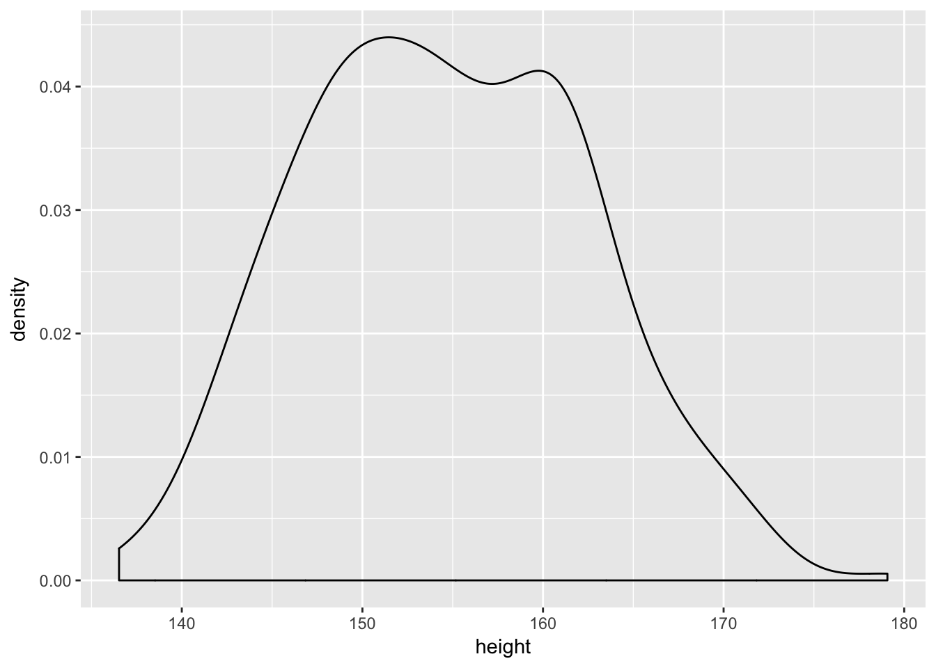
But be careful about choosing the Gaussian distribution only when the plotted outcome variable looks Gaussian to you. Gawking at the raw data, to try to decide how to model them, is usually not a good idea. The data could be a mixture of different Gaussian distributions, for example, and in that case you won’t be able to detect the underlying normality just by eyeballing the outcome distribution. Furthermore, the empirical distribution needn’t be actually Gaussian in order to justify using a Gaussian likelihood.
Consider the model:
\[\begin{eqnarray} { h }_{ i } & \sim & Normal(\mu ,\sigma ) & \text{<- likelihood} \\ \mu & \sim & Normal(178,20) & \text{<- } \mu \text{ prior} \\ \sigma & \sim & Cauchy(0,1) & \text{<- } \sigma \text{ prior} \end{eqnarray}\]
The short model above is sometimes described as assuming that the values \({ h }_{ i }\) are independent and identically distributed (i.e. i.i.d., iid, or IID). “iid” indicates that each value \({ h }_{ i }\) has the same probability function, independent of the other \(h\) values and using the same parameters. A moment’s reflection tells us that this is hardly ever true, in a physical sense. Whether measuring the same distance repeatedly or studying a population of heights, it is hard to argue that every measurement is independent of the others. The i.i.d. assumption doesn’t have to seem awkward, however, as long as you remember that probability is inside the golem, not outside in the world. The i.i.d. assumption is about how the golem represents its uncertainty. It is an epistemological assumption. It is not a physical assumption about the world, an ontological one, unless you insist that it is.
There’s no reason to expect a hard upper bound on (\sigma).
# Plot prior for mu
prior_mu <- ggplot(data = tibble(x = seq(from = 100, to = 250, by = .1)),
                   aes(x = x, y = dnorm(x, mean = 178, sd = 20))) +
    geom_line() +
    xlab(expression(mu)) +
    ylab("density")

# Plot prior for sigma
prior_sigma <- ggplot(data = tibble(x = seq(from = -10, to = 60, by = 1)),
                      aes(x = x, y = dunif(x, min = 0, max = 50))) +
    geom_line() +
    scale_y_continuous(NULL, breaks = NULL) +
    xlab(expression(sigma))

# Plot heights by sampling from the prior
sample_mu <- rnorm(1e4, 178, 20)
sample_sigma <- runif(1e4, 0, 50)

heights <- tibble(x = rnorm(1e4, sample_mu, sample_sigma)) %>%
    ggplot(aes(x = x)) +
    geom_density() +
    scale_y_continuous(NULL, breaks = NULL) +
    xlab("h")

library(gridExtra)
grid.arrange(prior_mu, prior_sigma, heights, ncol=3)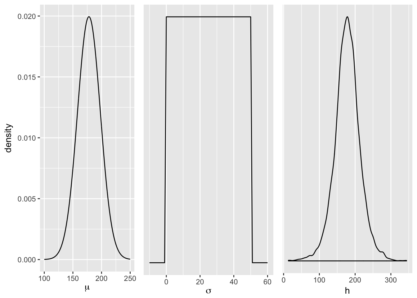
4.3.5. Fitting the model with brm
# Detach rethinking package
detach(package:rethinking, unload = T)

# Load brms
library(brms)
## Warning: package 'brms' was built under R version 3.4.4## Loading required package: Rcpp## Warning: package 'Rcpp' was built under R version 3.4.4## Loading 'brms' package (version 2.2.0). Useful instructions
## can be found by typing help('brms'). A more detailed introduction
## to the package is available through vignette('brms_overview').
## Run theme_set(theme_default()) to use the default bayesplot theme.# Construct the model and set the priors
m4.1 <- brm(data = d2, family = gaussian(),
height ~ 1,
prior = c(set_prior("normal(178, 20)", class = "Intercept"),
set_prior("cauchy(0, 1)", class = "sigma")),
chains = 4, iter = 2000, warmup = 1000, cores = 4)## Compiling the C++ model## Start sampling# Plot the chains
plot(m4.1)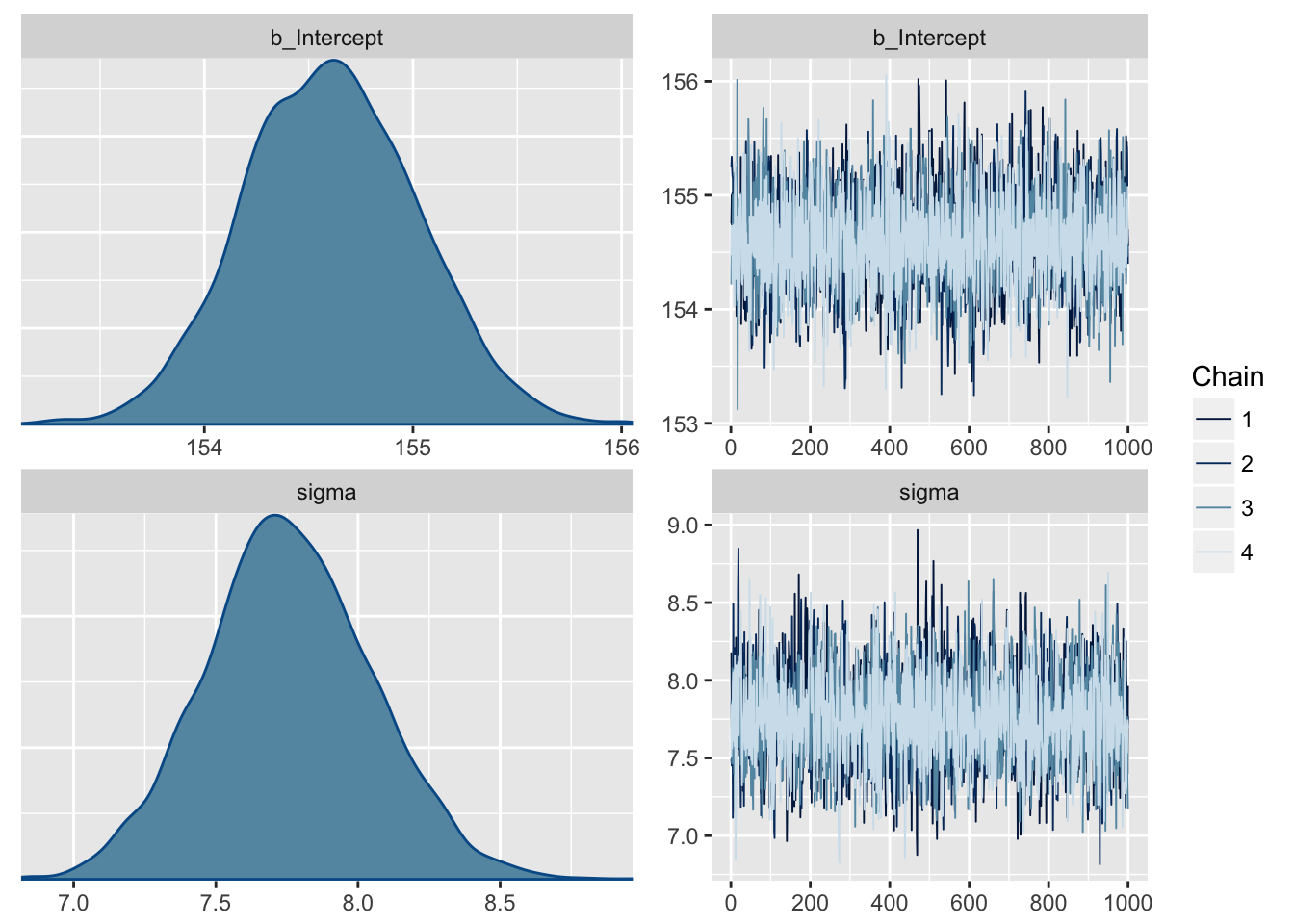
# Summarise the model
summary(m4.1, prob = 0.89)
## Family: gaussian
## Links: mu = identity; sigma = identity
## Formula: height ~ 1
## Data: d2 (Number of observations: 352)
## Samples: 4 chains, each with iter = 2000; warmup = 1000; thin = 1;
## total post-warmup samples = 4000
## ICs: LOO = NA; WAIC = NA; R2 = NA
##
## Population-Level Effects:
## Estimate Est.Error l-89% CI u-89% CI Eff.Sample Rhat
## Intercept 154.61 0.41 153.95 155.27 3368 1.00
##
## Family Specific Parameters:
## Estimate Est.Error l-89% CI u-89% CI Eff.Sample Rhat
## sigma 7.76 0.29 7.30 8.24 3692 1.00
##
## Samples were drawn using sampling(NUTS). For each parameter, Eff.Sample
## is a crude measure of effective sample size, and Rhat is the potential
## scale reduction factor on split chains (at convergence, Rhat = 1).Est.Error is equivalent to StdDev.
4.3.6. Sampling from a brm fit
# Extract the iterations of the HMC chains and put them in a data frame
post <- posterior_samples(m4.1)

# Summarise the samples
t(apply(post[ , 1:2], 2, quantile, probs = c(.5, .055, .945)))
## 50% 5.5% 94.5%
## b_Intercept 154.601479 153.951119 155.268724
## sigma 7.749569 7.299051 8.237449# Using the tidyverse for summarising
post %>%
select(-lp__) %>%
gather(parameter) %>%
group_by(parameter) %>%
summarise(mean = mean(value),
SD = sd(value),
`5.5_percentile` = quantile(value, probs = .055),
`94.5_percentile` = quantile(value, probs = .945)) %>%
mutate_if(is.numeric, round, digits = 2)## # A tibble: 2 x 5
## parameter mean SD `5.5_percentile` `94.5_percentile`
## <chr> <dbl> <dbl> <dbl> <dbl>
## 1 b_Intercept 155. 0.410 154. 155.
## 2 sigma 7.76 0.290 7.30 8.24# The rethinking package has already a function to summarise the samples
rethinking::precis(post[ , 1:2])## Mean StdDev |0.89 0.89|
## b_Intercept 154.61 0.41 153.98 155.28
## sigma 7.76 0.29 7.32 8.264.4. Adding a predictor
\[\begin{eqnarray} { h }_{ i } & \sim & Normal({ \mu }_{ i },\sigma ) & \text{<- likelihood } \\ { \mu }_{ i } & = & \alpha +\beta { x }_{ i } & \text{<- linear model} \\ \alpha & \sim & Normal(178,100) & \text{<- }\alpha \text{ prior } \\ \beta & \sim & Normal(0,10) & \text{<- }\beta \text{ prior } \\ \sigma & \sim & Cauchy(0,1) & \text{<- }\sigma \text{ prior } \end{eqnarray}\]
The linear model is asking two questions about the mean of the outcome:
- What is the expected height, when \(x_i = 0\)? The parameter \(\alpha\) answers this question. Parameters like \(\alpha\) are “intercepts” that tell us the value of \(\mu\) when all of the predictor variables have value zero. As a consequence, the value of the intercept is frequently uninterpretable without also studying any \(\beta\) parameters.
- What is the change in expected height, when \(x_i\) changes by 1 unit? The parameter \(\beta\) answers this question.
The prior for \(\beta\) places just as much probability below zero as it does above zero, and when \(\beta = 0\), weight has no relationship to height. Such a prior will pull probability mass towards zero, leading to more conservative estimates than a perfectly flat prior will.
What’s the correct prior? There is no more a uniquely correct prior than there is a uniquely correct likelihood. In choosing priors, there are simple guidelines to get you started. Priors encode states of information before seeing data. So priors allow us to explore the consequences of beginning with different information. In cases in which we have good prior information that discounts the plausibility of some parameter values, we can encode that information directly into priors. When we don’t have such information, we still usually know enough about the plausible range of values. And you can vary the priors and repeat the analysis in order to study how different states of initial information influence inference. Frequently, there are many reasonable choices for a prior, and all of them produce the same inference. And conventional Bayesian priors are conservative, relative to conventional non-Bayesian approaches.
4.4.2. Fitting the model
m4.3 <- brm(height ~ 1 + weight,
            data = d2,
            family = gaussian(),
            prior = c(set_prior("normal(178,100)", class = "Intercept"),
                      set_prior("normal(0,10)", class = "b"),
                      set_prior("cauchy(0,1)", class = "sigma")),
            chains = 4, iter = 41000, warmup = 40000, cores = 4)

plot(m4.3)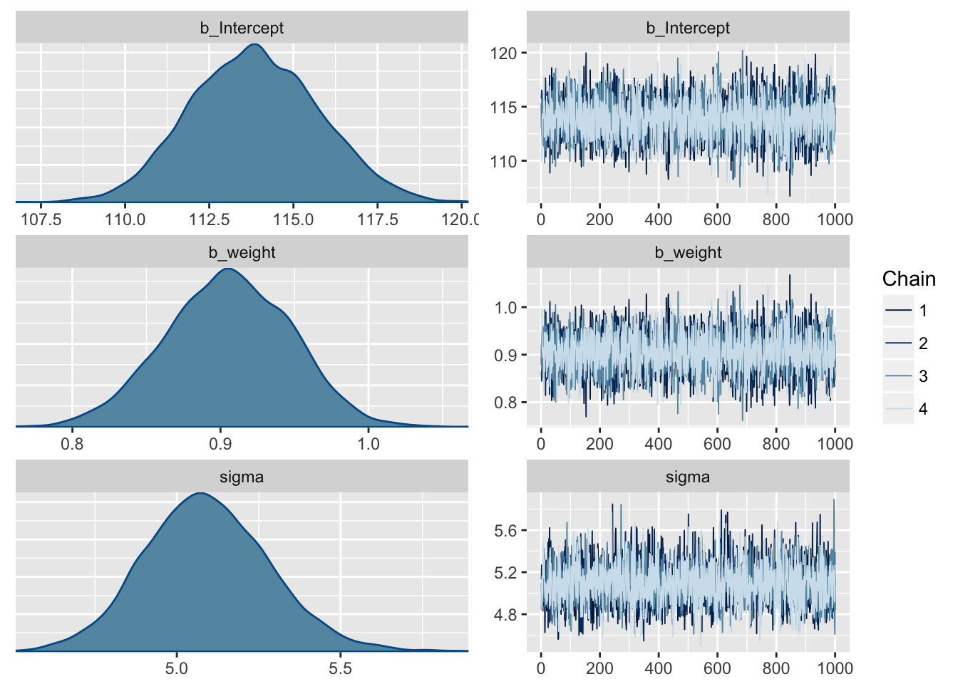
4.4.3. Interpreting the model fit
4.4.3.1. Tables of estimates
Posterior probabilities of parameter values describe the relative compatibility of different states of the world with the data, according to the model.
# Check the correlations among parameters
posterior_samples(m4.3) %>%
    select(-lp__) %>%
    cor() %>%
    round(digits = 2)
## b_Intercept b_weight sigma
## b_Intercept 1.00 -0.99 -0.01
## b_weight -0.99 1.00 0.02
## sigma -0.01 0.02 1.00pairs(m4.3)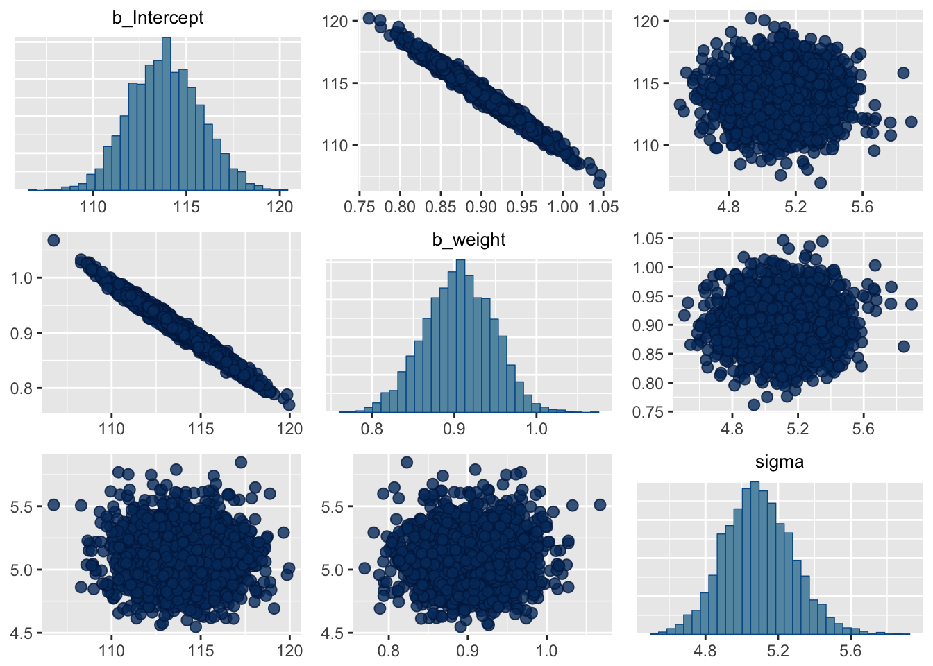
With centering, we can reduce the correlations among the parameters. Furthermore, by centering the predictor, the estimate for the intercept \(\alpha\) corresponds to the expected value of the outcome, when the predictor is at its average value.
d3 <- d2 %>%
    mutate(weight.c = weight - mean(weight))

m4.4 <- brm(height ~ 1 + weight.c,
            data = d3,
            family = gaussian(), # default
            prior = c(set_prior("normal(178,100)", class = "Intercept"),
                      set_prior("normal(0,10)", class = "b"),
                      set_prior("cauchy(0,1)", class = "sigma")),
            chains = 4, iter = 41000, warmup = 40000, cores = 4)

plot(m4.4)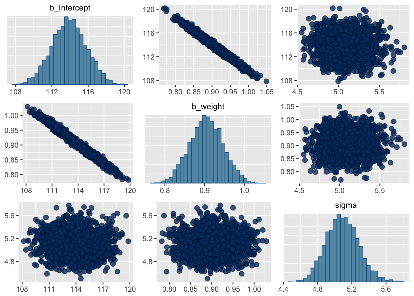
posterior_samples(m4.4) %>%
  select(-lp__) %>%
  gather(parameter) %>%
  group_by(parameter) %>%
  summarise(mean = mean(value),
            SD   = sd(value),
            `5.5_percentile`  = quantile(value, probs = .055),
            `94.5_percentile` = quantile(value, probs = .945)) %>%
  mutate_if(is.numeric, round, digits = 2)
## # A tibble: 3 x 5
## parameter mean SD `5.5_percentile` `94.5_percentile`
## <chr> <dbl> <dbl> <dbl> <dbl>
## 1 b_Intercept 155. 0.270 154. 155.
## 2 b_weight.c 0.900 0.0400 0.840 0.970
## 3 sigma 5.09 0.190 4.79 5.41posterior_samples(m4.4) %>%
select(-lp__) %>%
cor() %>%
round(digits = 2)## b_Intercept b_weight.c sigma
## b_Intercept 1.00 -0.01 0.00
## b_weight.c -0.01 1.00 -0.01
## sigma 0.00 -0.01 1.00pairs(m4.4)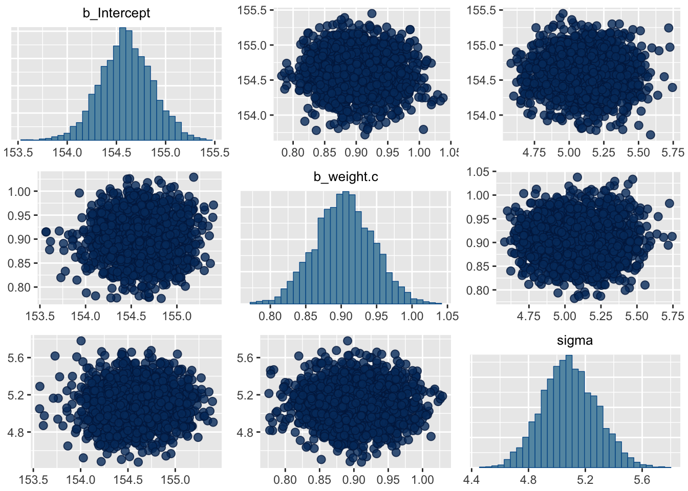
4.4.3.2. Plotting posterior inference against the data
d2 %>%
    ggplot(aes(x = weight, y = height)) +
    theme_bw() +
    geom_abline(intercept = fixef(m4.3)[1],
                slope = fixef(m4.3)[2]) +
  geom_point(shape = 1, size = 2, color = "royalblue") +
  theme(panel.grid = element_blank())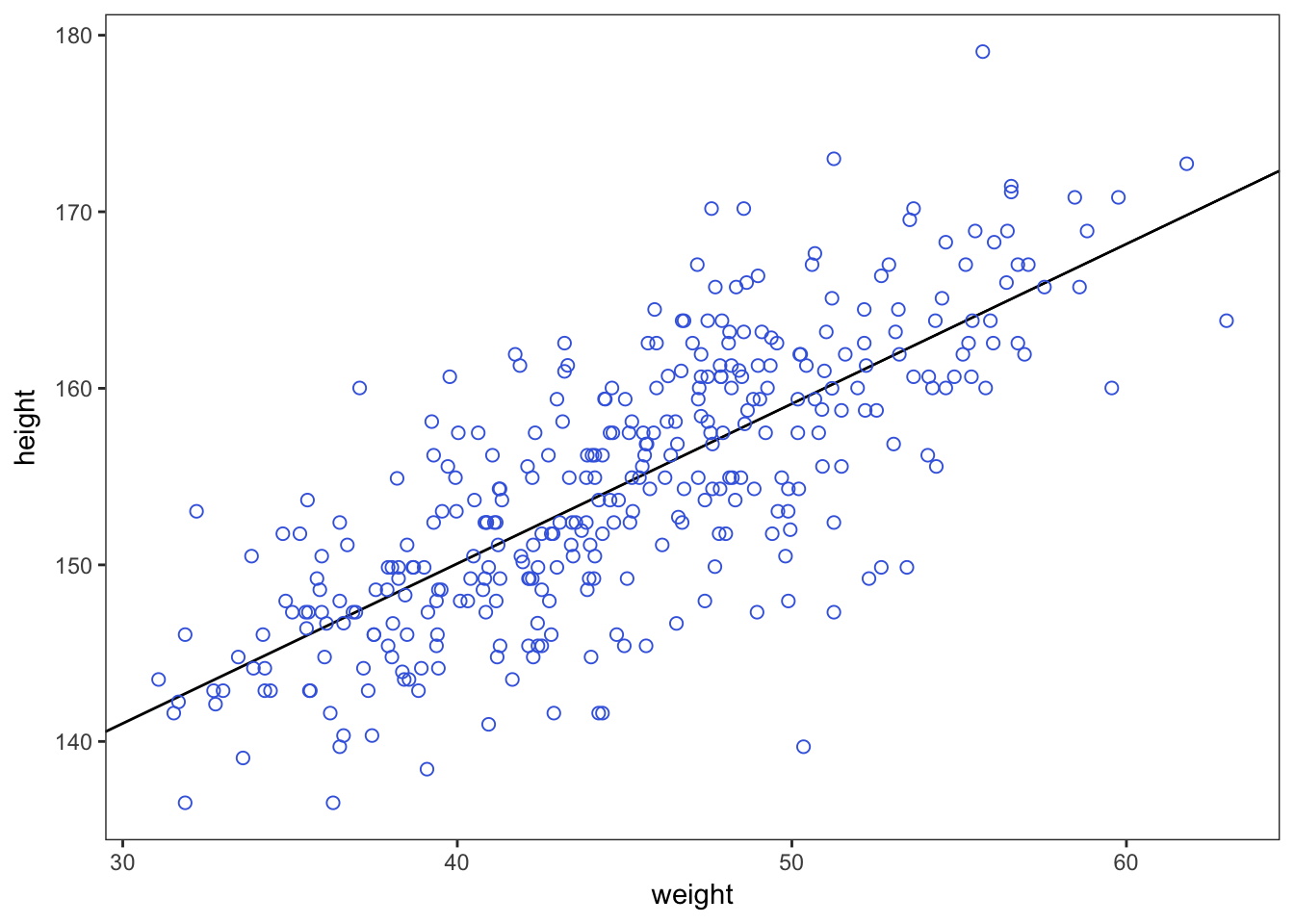
4.4.3.4. Plotting regression intervals and contours
brms::fitted() is the anologue to rethinking::link().
# When you specify summary = F, fitted() returns a matrix of values with as many rows as there were post-warmup iterations across your HMC chains and as many columns as there were cases in your analysis.
mu <- fitted(m4.3, summary = F)

# Plot regression line and its intervals
weight_seq <- tibble(weight = seq(from = 25, to = 70, by = 1))
muSummary <- fitted(m4.3,
                    newdata = weight_seq,
                    probs = c(0.055, 0.945)) %>%
    as_tibble() %>%
    bind_cols(weight_seq) %>%
    walk(head)

d2 %>%
    ggplot(aes(x = weight, y = height)) +
    geom_ribbon(data = muSummary,
                aes(y = Estimate, ymin = `5.5%ile`, ymax = `94.5%ile`),
                fill = "grey70") +
    geom_line(data = muSummary,
              aes(y = Estimate),
              color = "red") +
    geom_point(color = "navyblue", shape = 1, size = 1.5, alpha = 2/3) +
    theme(text = element_text(family = "Times"),
          panel.grid = element_blank())
## Warning: Ignoring unknown aesthetics: y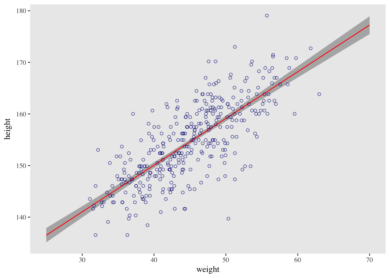
4.4.3.5. Prediction intervals
brms::predict() is the anologue to rethinking::sim().
# The summary information in our data frame is for simulated heights, not distributions of plausible average height, $\mu$
pred_height <- predict(m4.3,
                       newdata = weight_seq,
                       probs = c(0.055, 0.945)) %>%
    as_tibble() %>%
    bind_cols(weight_seq)

d2 %>%
    ggplot(aes(x = weight, y = height)) +
    geom_ribbon(data = pred_height,
                aes(y = Estimate, ymin = `5.5%ile`, ymax = `94.5%ile`),
                fill = "grey83") +
    geom_ribbon(data = muSummary,
                aes(y = Estimate, ymin = `5.5%ile`, ymax = `94.5%ile`),
                fill = "grey70") +
    geom_line(data = muSummary,
              aes(y = Estimate),
              color = "red") +
    geom_point(color = "navyblue", shape = 1, size = 1.5, alpha = 2/3) +
    theme(text = element_text(family = "Times"),
          panel.grid = element_blank())
## Warning: Ignoring unknown aesthetics: y
## Warning: Ignoring unknown aesthetics: y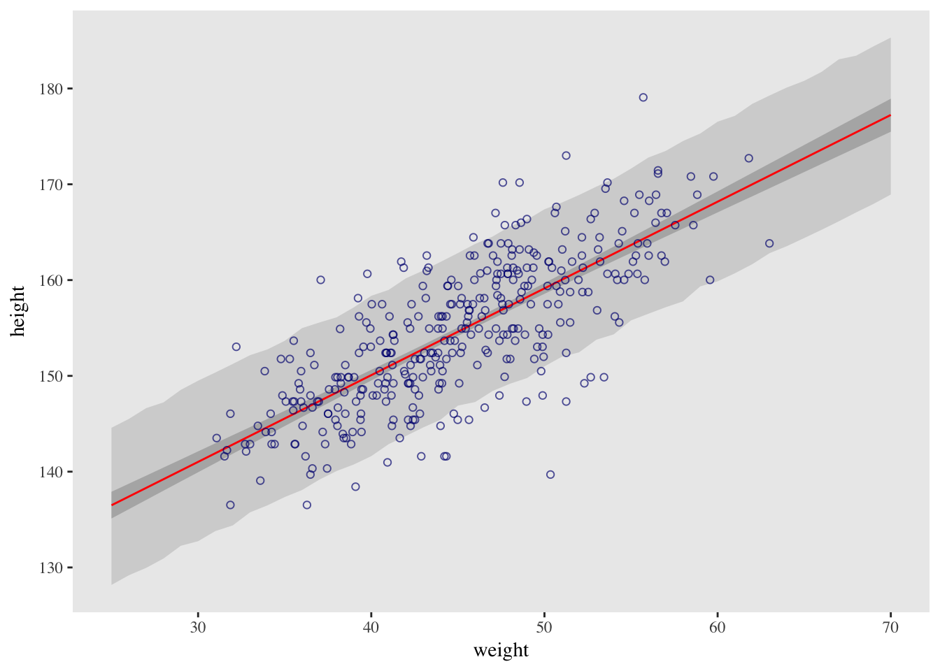
The outline for the wide shaded interval is a little jagged. This is the simulation variance in the tails of the sampled Gaussian values. Increase the number of samples to reduce it. With extreme percentiles, it can be very hard to get out all of the jaggedness.
Two kinds of uncertainty. In the procedure above, we encountered both uncertainty in parameter values and uncertainty in a sampling process. These are distinct concepts, even though they are processed much the same way and end up blended together in the posterior predictive simulation (check Chapter 3). The posterior distribution is a ranking of the relative plausibilities of every possible combination of parameter values. The distribution of simulated outcomes is instead a distribution that includes sampling variation from some process that generates Gaussian random variables. This sampling variation is still a model assumption. It’s no more or less objective than the posterior distribution. Both kinds of uncertainty matter, at least sometimes. But it’s important to keep them straight, because they depend upon different model assumptions. Furthermore, it’s possible to view the Gaussian likelihood as a purely epistemological assumption (a device for estimating the mean and variance of a variable), rather than an ontological assumption about what future data will look like. In that case, it may not make complete sense to simulate outcomes.
4.5. Polynomial regression
In general, it’s not good to use polynomial regression because polynomials are very hard to interpret. Better would be to have a more mechanistic model of the data, one that builds the non-linear relationship up from a principled beginning.
Standarization of a predictor means to first center the variable and then divide it by its standard deviation. This leaves the mean at zero but also rescales the range of the data. This is helpful for two reasons:
- Interpretation might be easier. For a standardized variable, a change of one unit is equivalent to a change of one standard deviation. In many contexts, this is more interesting and more revealing than a one unit change on the natural scale. And once you start making regressions with more than one kind of predictor variable, standardizing all of them makes it easier to compare their relative influence on the outcome, using only estimates. On the other hand, you might want to interpret the data on the natural scale. So standardization can make interpretation harder, not easier.
- More important though are the advantages for fitting the model to the data. When predictor variables have very large values in them, there are sometimes numerical glitches. Even well-known statistical software can suffer from these glitches, leading to mistaken estimates. These problems are very common for polynomial regression, because the square or cube of a large number can be truly massive. Standardizing largely resolves this issue.
d <-
  d %>%
  mutate(weight.s = (weight - mean(weight))/sd(weight),
         weight.s2 = weight.s^2)
Consider the following parabolic model:
\[\begin{eqnarray} { h }_{ i } & \sim & Normal({ \mu }_{ i },\sigma ) & \text{<- likelihood } \\ { \mu }_{ i } & = & \alpha +{ \beta }_{ 1 }{ x }_{ i }+{ \beta }_{ 2 }{ x }_{ i }^{ 2 } & \text{<- linear model } \\ \alpha & \sim & Normal(178,100) & \text{<- }\alpha \text{ prior } \\ { \beta }_{ 1 } & \sim & Normal(0,10) & \text{<- }{ \beta }_{ 1 }\text{ prior } \\ { \beta }_{ 2 } & \sim & Normal(0,10) & \text{<- }{ \beta }_{ 2 } \text{ prior} \\ \sigma & \sim & Cauchy(0,1) & \text{<- }\sigma \text{ prior } \end{eqnarray}\]
d %>%
    ggplot(aes(x = weight.s, y = height)) +
    geom_point(color = "navyblue", shape = 1, size = 1.5)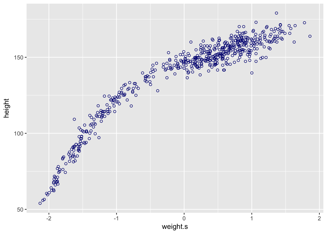
m4.5 <- brm(height ~ 1 + weight.s + I(weight.s^2),
            data = d,
            prior = c(set_prior("normal(178,100)", class = "Intercept"),
                      set_prior("normal(0,10)", class = "b"),
                      set_prior("cauchy(0,1)", class = "sigma")),
            chains = 4, iter = 2000, warmup = 1000, cores = 4)

plot(m4.5)
posterior_samples(m4.5) %>%
  select(-lp__) %>%
  gather(parameter) %>%
  group_by(parameter) %>%
  summarise(mean = mean(value),
            SD   = sd(value),
            `5.5_percentile`  = quantile(value, probs = .055),
            `94.5_percentile` = quantile(value, probs = .945)) %>%
  mutate_if(is.numeric, round, digits = 2)
## # A tibble: 4 x 5
## parameter mean SD `5.5_percentile` `94.5_percentile`
## <chr> <dbl> <dbl> <dbl> <dbl>
## 1 b_Intercept 147. 0.360 146. 147.
## 2 b_Iweight.sE2 -8.42 0.270 -8.85 -7.99
## 3 b_weight.s 21.4 0.280 20.9 21.8
## 4 sigma 5.77 0.180 5.49 6.06posterior_samples(m4.5) %>%
select(-lp__) %>%
cor() %>%
round(digits = 2)## b_Intercept b_weight.s b_Iweight.sE2 sigma
## b_Intercept 1.00 -0.36 -0.74 0.02
## b_weight.s -0.36 1.00 0.49 -0.04
## b_Iweight.sE2 -0.74 0.49 1.00 -0.03
## sigma 0.02 -0.04 -0.03 1.00pairs(m4.5)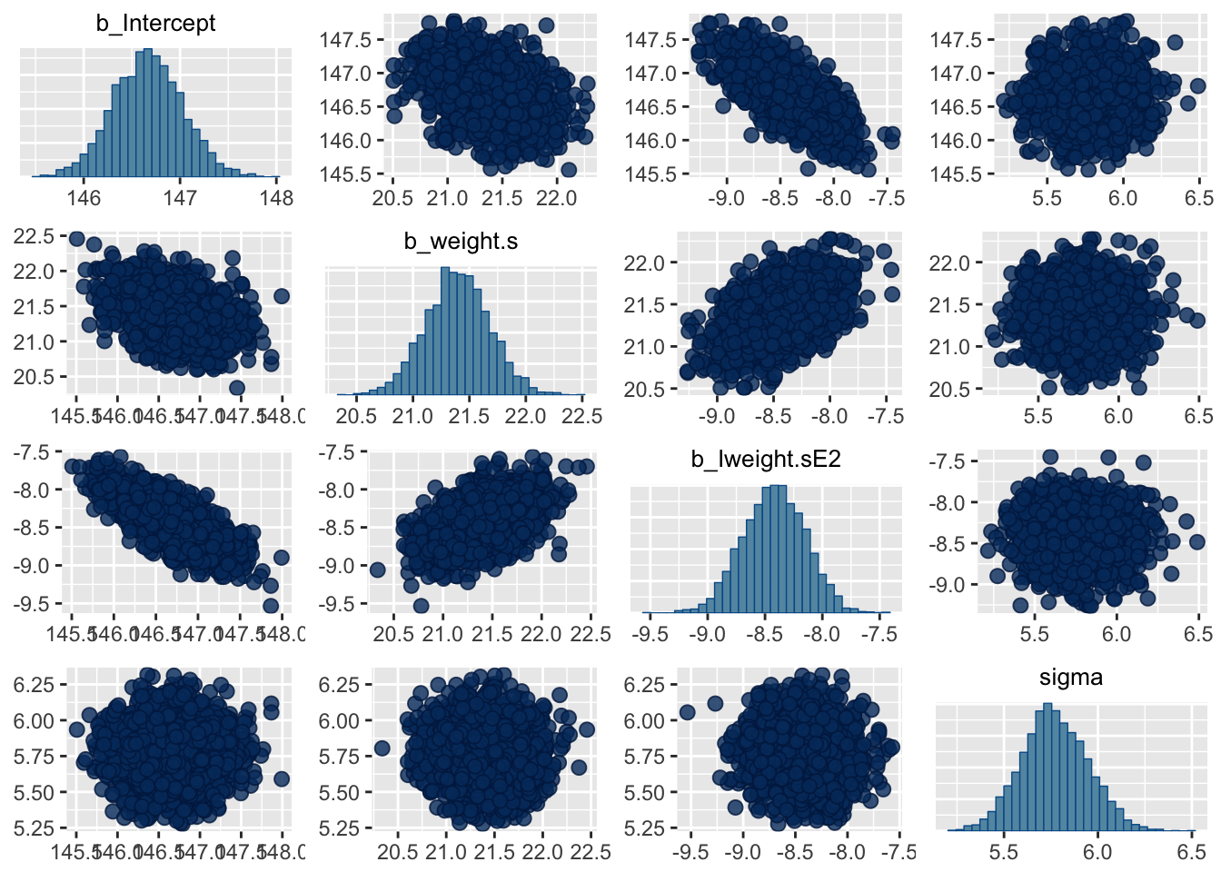
weight_seq <- data.frame(weight.s = seq(from = -2.2, to = 2, length.out = 30))

muSummary <- fitted(m4.5,
                    newdata = weight_seq,
                    probs = c(0.055, 0.945)) %>%
    as_tibble() %>%
    bind_cols(weight_seq)

pred_height <- predict(m4.5,
                       newdata = weight_seq,
                       probs = c(0.055, 0.945)) %>%
    as_tibble() %>%
    bind_cols(weight_seq)

d %>%
    ggplot(aes(x = weight.s, y = height)) +
    geom_ribbon(data = pred_height,
                aes(y = Estimate, ymin = `5.5%ile`, ymax = `94.5%ile`),
                fill = "grey83") +
    geom_ribbon(data = muSummary,
                aes(y = Estimate, ymin = `5.5%ile`, ymax = `94.5%ile`),
                fill = "grey70") +
    geom_line(data = muSummary,
              aes(y = Estimate),
              color = "red") +
    geom_point(color = "navyblue", shape = 1, size = 1.5, alpha = 2/3) +
    theme(text = element_text(family = "Times"),
          panel.grid = element_blank())
## Warning: Ignoring unknown aesthetics: y
## Warning: Ignoring unknown aesthetics: y
# Correct the x scale
at <- c(-2, -1, 0, 1, 2)

d %>%
    ggplot(aes(x = weight.s, y = height)) +
    geom_ribbon(data = pred_height,
                aes(y = Estimate, ymin = `5.5%ile`, ymax = `94.5%ile`),
                fill = "grey83") +
    geom_ribbon(data = muSummary,
                aes(y = Estimate, ymin = `5.5%ile`, ymax = `94.5%ile`),
                fill = "grey70") +
    geom_line(data = muSummary,
              aes(y = Estimate),
              color = "red") +
    geom_point(color = "navyblue", shape = 1, size = 1.5, alpha = 2/3) +
    theme(text = element_text(family = "Times"),
          panel.grid = element_blank()) +
    # Here it is!
    scale_x_continuous(breaks = at,
                       labels = round(at*sd(d$weight) + mean(d$weight), 1))
## Warning: Ignoring unknown aesthetics: y
## Warning: Ignoring unknown aesthetics: y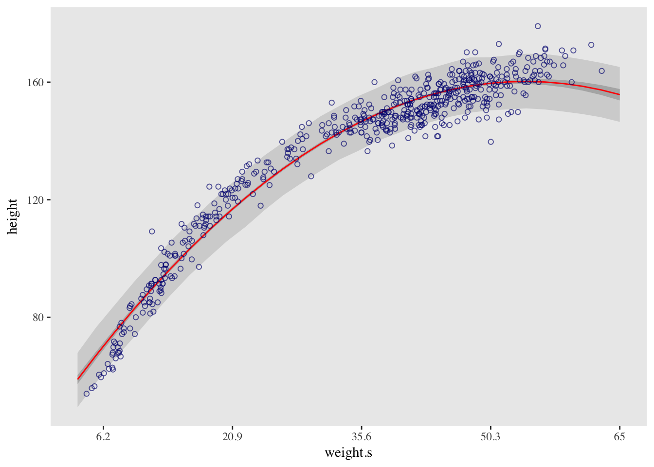
References
McElreath, R. (2016). Statistical rethinking: A Bayesian course with examples in R and Stan. Chapman & Hall/CRC Press.
Kurz, A. S. (2018, March 9). brms, ggplot2 and tidyverse code, by chapter. Retrieved from https://goo.gl/JbvNTj