Multivariate regression can be useful for several reasons:
- Statistical “control” for confounds. A confound is a variable that may be correlated with another variable of interest. Confounds can hide real important variables just as easily as they can produce false ones.
- Multiple causation. Even when confounds are absent, due for example to tight experimental control, a phenomenon may really arise from multiple causes. Measurement of each cause is useful, so when we can use the same data to estimate more than one type of influence, we should. Furthermore, when causation is multiple, one cause can hide another. Multivariate models can help in such settings.
- Interactions. Even when variables are completely uncorrelated, the importance of each may still depend upon the other. For example, plants benefit from both light and water. But in the absence of either, the other is no benefit at all. Such interactions occur in a very large number of systems. So effective inference about one variable will usually depend upon consideration of other variables.
5.1. Spurious association
library(rethinking)
data(WaffleDivorce)
d <- WaffleDivorce

rm(WaffleDivorce)
detach(package:rethinking, unload = T)
library(brms)
## Warning: package 'brms' was built under R version 3.4.4## Warning: package 'Rcpp' was built under R version 3.4.4library(tidyverse)
glimpse(d)## Observations: 50
## Variables: 13
## $ Location <fct> Alabama, Alaska, Arizona, Arkansas, Californ...
## $ Loc <fct> AL, AK, AZ, AR, CA, CO, CT, DE, DC, FL, GA, ...
## $ Population <dbl> 4.78, 0.71, 6.33, 2.92, 37.25, 5.03, 3.57, 0...
## $ MedianAgeMarriage <dbl> 25.3, 25.2, 25.8, 24.3, 26.8, 25.7, 27.6, 26...
## $ Marriage <dbl> 20.2, 26.0, 20.3, 26.4, 19.1, 23.5, 17.1, 23...
## $ Marriage.SE <dbl> 1.27, 2.93, 0.98, 1.70, 0.39, 1.24, 1.06, 2....
## $ Divorce <dbl> 12.7, 12.5, 10.8, 13.5, 8.0, 11.6, 6.7, 8.9,...
## $ Divorce.SE <dbl> 0.79, 2.05, 0.74, 1.22, 0.24, 0.94, 0.77, 1....
## $ WaffleHouses <int> 128, 0, 18, 41, 0, 11, 0, 3, 0, 133, 381, 0,...
## $ South <int> 1, 0, 0, 1, 0, 0, 0, 0, 0, 1, 1, 0, 0, 0, 0,...
## $ Slaves1860 <int> 435080, 0, 0, 111115, 0, 0, 0, 1798, 0, 6174...
## $ Population1860 <int> 964201, 0, 0, 435450, 379994, 34277, 460147,...
## $ PropSlaves1860 <dbl> 4.5e-01, 0.0e+00, 0.0e+00, 2.6e-01, 0.0e+00,...Multivariate models ask the following question: What is the predictive value of a variable, once I already know all of the other predictor variables?
5.1.1. Multivariate notation
Consider the following multivariate model where \(R_i\) is marriage rate (Marriage.s), \(A_i\) is median age at marriage (MedianAgeMarriage.s) and \(D_i\) is divorce rate:
\[\begin{eqnarray} { D }_{ i } & \sim & \text{Normal}({ \mu }_{ i },\sigma ) & \text{<- likelihood } \\ { \mu }_{ i } & = & \alpha +{ \beta }_{ R }{ R }_{ i }+{ \beta }_{ A}{ A }_{ i } & \text{<- linear model } \\ \alpha & \sim & \text{Normal}(10,10) & \text{<- }\alpha \text{ prior } \\ { \beta }_{ R } & \sim & \text{Normal}(0,1) & \text{<- }{ \beta }_{ R }\text{ prior } \\ { \beta }_{ A } & \sim & \text{Normal}(0,1) & \text{<- }{ \beta }_{ A } \text{ prior} \\ \sigma & \sim & \text{Cauchy}(0,1) & \text{<- }\sigma \text{ prior } \end{eqnarray}\]
What does it mean \({ \mu }_{ i } = \alpha +{ \beta }_{ R }{ R }_{ i }+{ \beta }_{ A}{ A }_{ i }\)? It can be interpreted as: A State’s divorce rate can be a function of its marriage rate or its median age at marriage. The “or” indicates independent associations, which may be purely statistical or rather causal.
5.1.2. Fitting the model
d <-
    d %>%
    mutate(Marriage.s = (Marriage - mean(Marriage))/sd(Marriage),
           MedianAgeMarriage.s = (MedianAgeMarriage - mean(MedianAgeMarriage))/sd(MedianAgeMarriage))

m5.3 <- brm(Divorce ~ 1 + Marriage.s + MedianAgeMarriage.s,
            data = d,
            prior = c(set_prior("normal(10,10)", class = "Intercept"),
                      set_prior("normal(0,1)", class = "b"),
                      set_prior("cauchy(0,1)", class = "sigma")),
            chains = 4, iter = 2000, warmup = 500, cores = 4)

summary(m5.3, prob = 0.89)
## Family: gaussian
## Links: mu = identity; sigma = identity
## Formula: Divorce ~ 1 + Marriage.s + MedianAgeMarriage.s
## Data: d (Number of observations: 50)
## Samples: 4 chains, each with iter = 2000; warmup = 500; thin = 1;
## total post-warmup samples = 6000
## ICs: LOO = NA; WAIC = NA; R2 = NA
##
## Population-Level Effects:
## Estimate Est.Error l-89% CI u-89% CI Eff.Sample Rhat
## Intercept 9.69 0.21 9.35 10.03 5609 1.00
## Marriage.s -0.13 0.29 -0.59 0.34 4048 1.00
## MedianAgeMarriage.s -1.13 0.29 -1.59 -0.67 3891 1.00
##
## Family Specific Parameters:
## Estimate Est.Error l-89% CI u-89% CI Eff.Sample Rhat
## sigma 1.50 0.16 1.27 1.76 4854 1.00
##
## Samples were drawn using sampling(NUTS). For each parameter, Eff.Sample
## is a crude measure of effective sample size, and Rhat is the potential
## scale reduction factor on split chains (at convergence, Rhat = 1).stanplot(m5.3)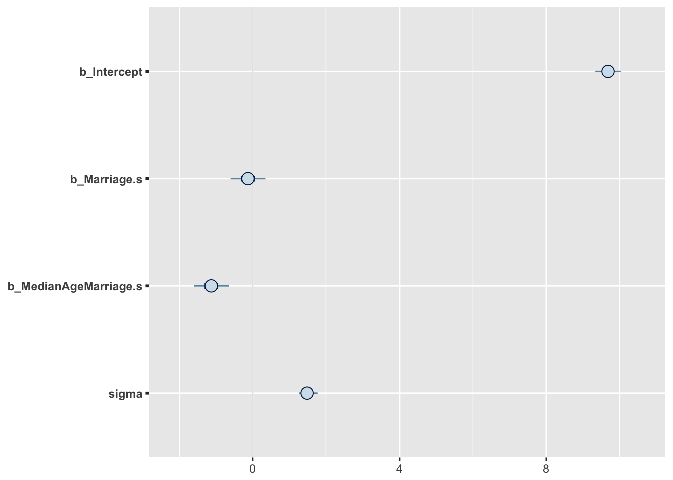
It’s worth checking the bayesplot package.
post <- posterior_samples(m5.3)

bayesplot::color_scheme_set("red")
bayesplot::mcmc_intervals(post[, 1:4],
                          prob = .5,
                          point_est = "median") +
  labs(title = "Coefficient plot") +
  theme(axis.text.y = element_text(hjust = 0),
        axis.line.x = element_line(size = 1/4),
        axis.line.y = element_blank(),
        axis.ticks.y = element_blank())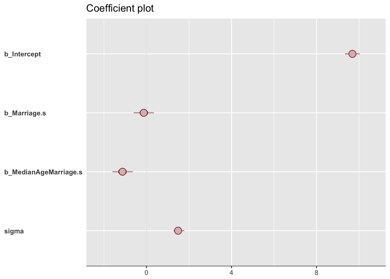
bayesplot::mcmc_areas(post[, 1:4],
                      prob = 0.8, # 80% intervals
                      prob_outer = 0.99, # 99%
                      point_est = "median"
)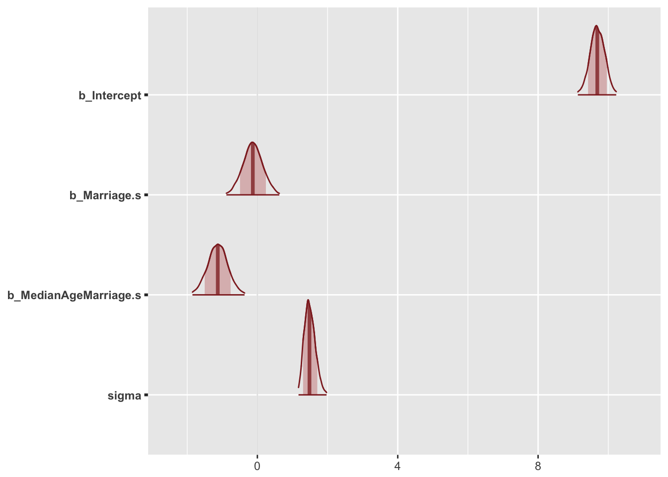
From the picture, it can be concluded that once we know median age at marriage for a State, there is little or no additional predictive power in also knowing the rate of marriage in that State. Note that this does not mean that there is no value in knowing marriage rate. If you didn’t have access to age-at-marriage data, then you’d definitely find value in knowing the marriage rate.
5.1.3. Plotting multivariate posteriors
There are a variety of plotting techniques that attempt to help one understand multiple linear regression. None of these techniques is suitable for all jobs, and most do not generalize beyond linear regression. Some interpretative plots for multivariate models are:
- Predictor residual plots. These plots show the outcome against residual predictor values.
- Counterfactual plots. These show the implied predictions for imaginary experiments in which the different predictor variables can be changed independently of one another.
- Posterior prediction plots. These show model-based predictions against raw data, or otherwise display the error in prediction.
5.1.3.1. Predictor residual plots
A predictor variable residual is the average prediction error when we use all of the other predictor variables to model a predictor of interest.
\[\begin{eqnarray} { R }_{ i } & \sim & \text{Normal}({ \mu }_{ i },\sigma ) & \text{<- likelihood } \\ { \mu }_{ i } & = & \alpha +{ \beta }_{ A}{ A }_{ i } & \text{<- linear model } \\ \alpha & \sim & \text{Normal}(0,10) & \text{<- }\alpha \text{ prior } \\ { \beta }_{ A } & \sim & \text{Normal}(0,1) & \text{<- }{ \beta }_{ A } \text{ prior} \\ \sigma & \sim & \text{Cauchy}(0,1) & \text{<- }\sigma \text{ prior } \end{eqnarray}\]
m5.4 <- brm(Marriage.s ~ 1 + MedianAgeMarriage.s,
            data = d,
            prior = c(set_prior("normal(0,10)", class = "Intercept"),
                      set_prior("normal(0,1)", class = "b"),
                      set_prior("cauchy(0,1)", class = "sigma")),
            chains = 4, iter = 2000, warmup = 500, cores = 4)

summary(m5.4, prob = 0.89)
## Family: gaussian
## Links: mu = identity; sigma = identity
## Formula: Marriage.s ~ 1 + MedianAgeMarriage.s
## Data: d (Number of observations: 50)
## Samples: 4 chains, each with iter = 2000; warmup = 500; thin = 1;
## total post-warmup samples = 6000
## ICs: LOO = NA; WAIC = NA; R2 = NA
##
## Population-Level Effects:
## Estimate Est.Error l-89% CI u-89% CI Eff.Sample Rhat
## Intercept 0.00 0.10 -0.16 0.16 5025 1.00
## MedianAgeMarriage.s -0.72 0.10 -0.87 -0.56 5681 1.00
##
## Family Specific Parameters:
## Estimate Est.Error l-89% CI u-89% CI Eff.Sample Rhat
## sigma 0.71 0.07 0.61 0.84 5430 1.00
##
## Samples were drawn using sampling(NUTS). For each parameter, Eff.Sample
## is a crude measure of effective sample size, and Rhat is the potential
## scale reduction factor on split chains (at convergence, Rhat = 1).df54 <-
residuals(m5.4) %>%
as_tibble() %>%
select(Estimate) %>%
bind_cols(d %>% select(Divorce))
ggplot(data = df54,
aes(x = Estimate, y = Divorce)) +
theme_bw() +
stat_smooth(method = "lm", color = "firebrick4", fill = "firebrick4",
alpha = 1/5, size = 1/2) +
geom_vline(xintercept = 0, linetype = 2, color = "grey50") +
geom_point(size = 2, color = "firebrick4", alpha = 2/3) +
coord_cartesian(ylim = c(6, 14.1)) +
annotate("text", x = -.14, y = 14.1, label = "younger older") +
labs(x = "Age of marriage residuals") +
theme(panel.grid = element_blank()) 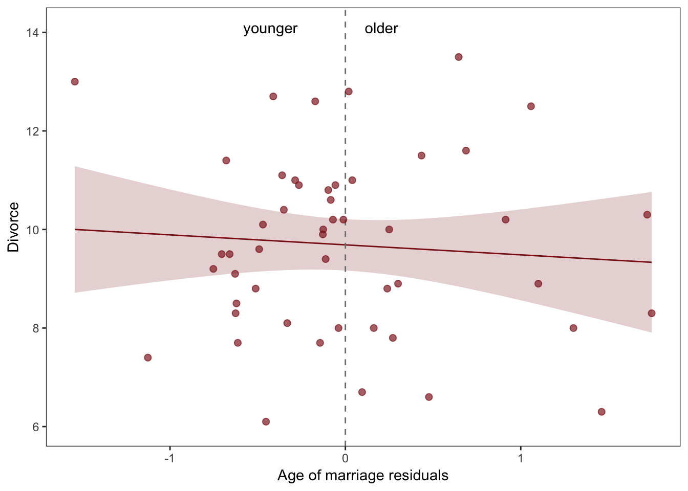
When a residual is positive, that means that the observed rate was in excess of what we’d expect, given the median age at marriage in that State. When a residual is negative, that means the observed rate was below what we’d expect. In simpler terms, States with positive residuals marry fast for their age of marriage, while States with negative residuals marry slow for their age of marriage.
The last plot displays the linear relationship between divorce and marriage rates, having statistically “controlled” for median age of marriage. The vertical dashed line indicates marriage rate that exactly matches the expectation from median age at marriage. So States to the right of the line marry faster than expected. States to the left of the line marry slower than expected. Average divorce rate on both sides of the line is about the same, and so the regression line demonstrates little relationship between divorce and marriage rates.
5.1.3.2. Counterfactual plots
It displays the implied predictions of the model even for unobserved or impossible values of the predictor variables.
nd <-
  tibble(Marriage.s = seq(from = -3, to = 3, length.out = 30),
         MedianAgeMarriage.s = rep(mean(d$MedianAgeMarriage.s,
                                        times = 30)))

pred53.a <- predict(m5.3, newdata = nd)
fitd53.a <- fitted(m5.3, newdata = nd)

# This isn't the most tidyverse-centric way of doing things, but it just seemed easier to rely on the bracket syntax for this one
tibble(Divorce = fitd53.a[, 1],
       fll     = fitd53.a[, 3],
       ful     = fitd53.a[, 4],
       pll     = pred53.a[, 3],
       pul     = pred53.a[, 4]) %>%
  bind_cols(nd) %>%  # Note our use of the pipe, here. This allowed us to feed the tibble directly into ggplot2 without having to save it as an object.

  ggplot(aes(x = Marriage.s, y = Divorce)) +
  theme_bw() +
  geom_ribbon(aes(ymin = pll, ymax = pul),
              fill = "firebrick", alpha = 1/5) +
  geom_ribbon(aes(ymin = fll, ymax = ful),
              fill = "firebrick", alpha = 1/5) +
  geom_line(color = "firebrick4") +
  coord_cartesian(ylim = c(6, 14)) +
  labs(subtitle = "Counterfactual plot for which MedianAgeMarriage.s = 0") +
theme(panel.grid = element_blank()) 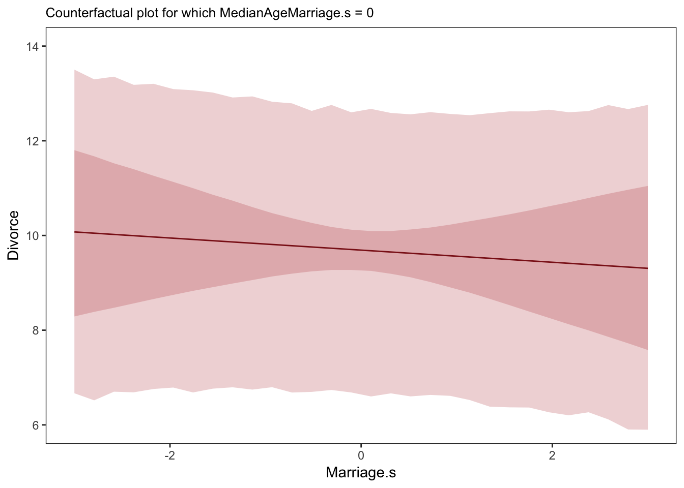
nd <-
  tibble(MedianAgeMarriage.s = seq(from = -3, to = 3.5, length.out = 30),
         Marriage.s = rep(mean(d$Marriage.s), times = 30))

pred53.b <- predict(m5.3, newdata = nd)
fitd53.b <- fitted(m5.3, newdata = nd)

tibble(Divorce = fitd53.b[, 1],
       fll     = fitd53.b[, 3],
       ful     = fitd53.b[, 4],
       pll     = pred53.b[, 3],
       pul     = pred53.b[, 4]) %>%
  bind_cols(nd) %>%
  ggplot(aes(x = MedianAgeMarriage.s, y = Divorce)) +
  theme_bw() +
  geom_ribbon(aes(ymin = pll, ymax = pul),
              fill = "firebrick", alpha = 1/5) +
  geom_ribbon(aes(ymin = fll, ymax = ful),
              fill = "firebrick", alpha = 1/5) +
  geom_line(color = "firebrick4") +
  coord_cartesian(ylim = c(6, 14)) +
  labs(subtitle = "Counterfactual plot for which Marriage.s = 0") +
theme(panel.grid = element_blank()) 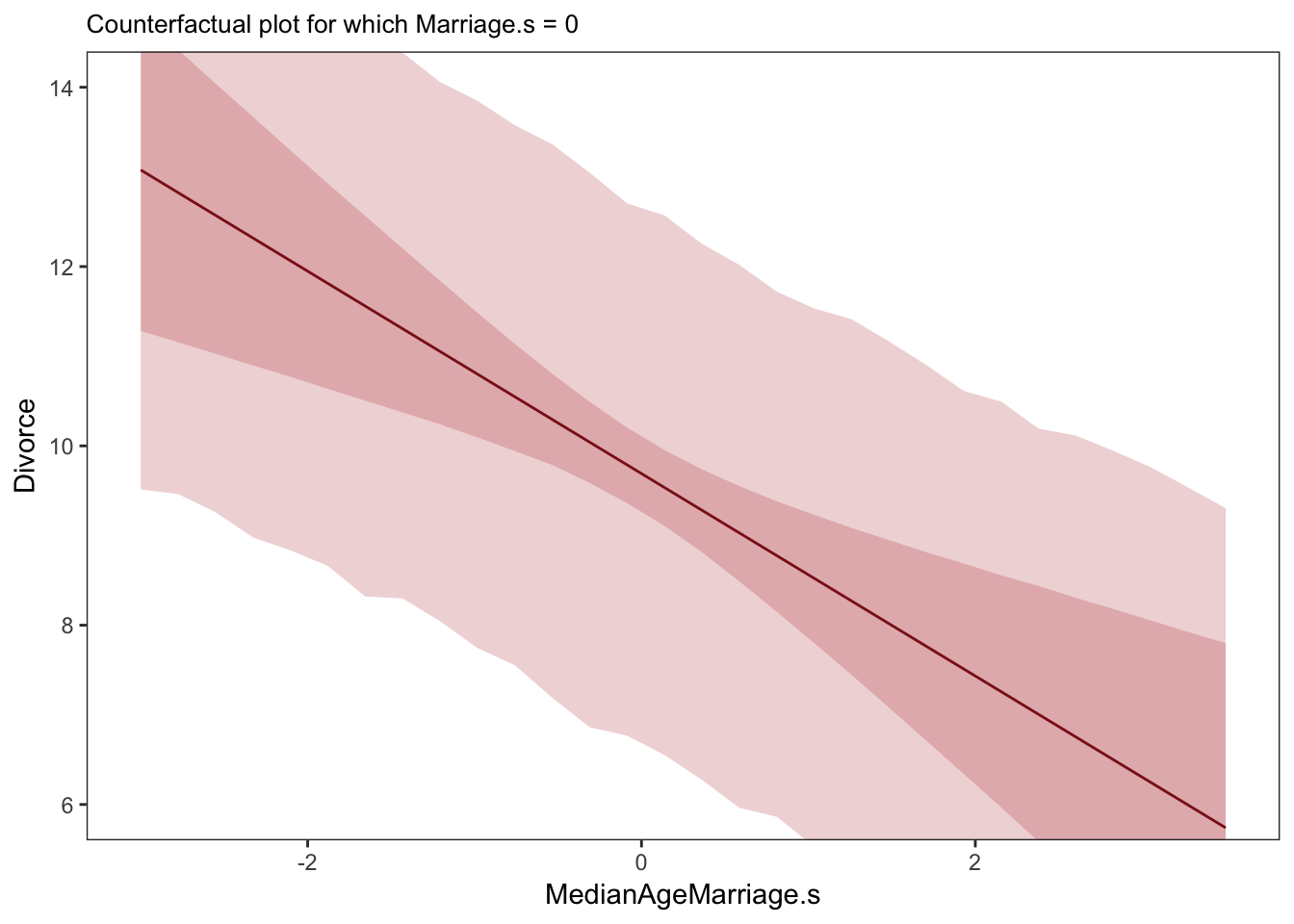
These plots have the same slopes as the residual plots in the previous section. But they don’t display any data, raw or residual, because they are counterfactual. And they also show percentile intervals on the scale of the data, instead of on that weird residual scale. As a result, they are direct displays of the impact on prediction of a change in each variable.
A tension with such plots, however, lies in their counterfactual nature. In the small world of the model, it is possible to change one feature without also changing another one. But is this also possible in the large world of reality? Probably not. In that case, while these counterfactual plots always help in understanding the model, they may also mislead by displaying predictions for impossible combinations of predictor values.
5.1.3.3. Posterior prediction plots
It’s important to check the model fit against the observed data.
# The thin lines are the 89% intervals and the thicker lines are +/- the posterior SD, both of which are returned with fitted()
fitted(m5.3, probs = c(0.055, 0.945)) %>%
    as_tibble() %>%
    bind_cols(d %>% select(Divorce, Loc)) %>%
    ggplot(aes(x = Divorce, y = Estimate)) +
    theme_bw() +
    geom_abline(linetype = 2, color = "grey50", size = .5) +
    geom_point(size = 1.5, color = "firebrick4", alpha = 3/4) +
    geom_linerange(aes(ymin = `5.5%ile`, ymax = `94.5%ile`),
                   size = 1/4, color = "firebrick4") +
    geom_linerange(aes(ymin = Estimate - Est.Error, ymax = Estimate + Est.Error),
                   size = 1/2, color = "firebrick4") +
    geom_text(data = . %>% filter(Loc %in% c("ID", "UT")),
              aes(label = Loc),
              hjust = 0, nudge_x = - 0.65) +
    labs(x = "Observed divorce", y = "Predicted divorce") +
    coord_fixed() +
    theme(panel.grid = element_blank())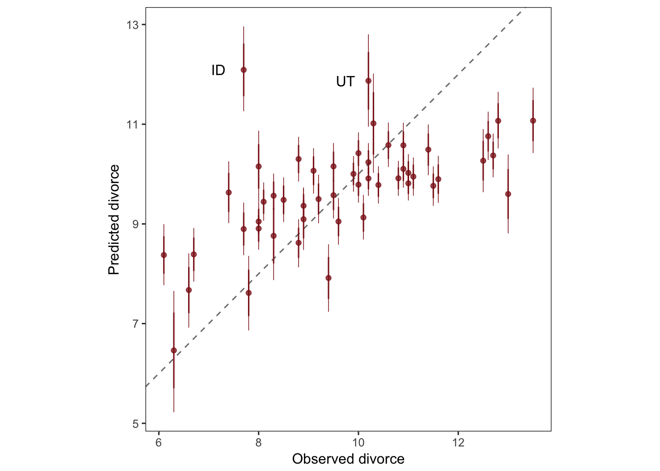
Residual plots show the mean prediction error for each row.
# This is for the average prediction error mean, +/- SD, and 95% intervals
res53 <-
  residuals(m5.3) %>%
  as_tibble() %>%
  bind_cols(d %>% select(Loc))

# This is the 95% prediction interval
pred53 <-
 predict(m5.3) %>%
  as_tibble() %>%
  transmute(`2.5%ile` = d$Divorce - `2.5%ile`,
            `97.5%ile` = d$Divorce - `97.5%ile`) %>%
  bind_cols(d %>% select(Loc))

# The plot
ggplot(data = res53,
       aes(x = reorder(Loc, Estimate), y = Estimate)) +
  theme_bw() +
  geom_hline(yintercept = 0, size = 1/2, color = "grey85") +
  geom_pointrange(aes(ymin = `2.5%ile`, ymax = `97.5%ile`),
                  size = 2/5, shape = 20, color = "firebrick4") +
  geom_segment(aes(y = Estimate - Est.Error,
                   yend = Estimate + Est.Error,
                   x = Loc, xend = Loc),
               size = 1, color = "firebrick4") +
  geom_segment(data = pred53,
               aes(y = `2.5%ile`, yend = `97.5%ile`,
                   x = Loc, xend = Loc),
               size = 3, color = "firebrick4", alpha = 1/10) +
  labs(x = NULL, y = "Divorce residuals") +
  coord_flip(ylim = c(-6, 5)) +
  theme(panel.grid = element_blank(),
        axis.ticks.y = element_blank(),
        axis.text.y = element_text(hjust = 0))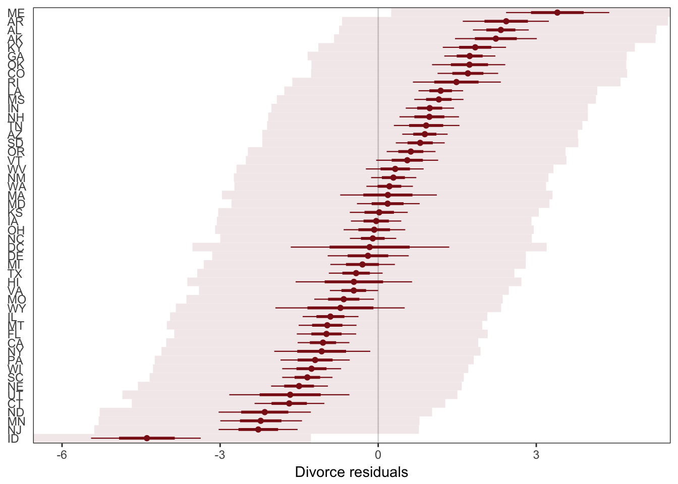
Common use for these simulations is to construct novel predictor residual plots. Once you’ve computed the outcome residuals you can plot those residuals against new predictor variables. This is a quick way to see if remaining variation in the outcome is associated with another predictor.
Keep in mind that no matter how many predictors you’ve already included in a regression, it’s still possible to find spurious correlations with the remaining variation.
All statistical models are vulnerable to and demand critique, regardless of the precision of their estimates and apparent accuracy of their predictions. Rounds of model criticism and revision embody the real tests of scientific hypotheses, while the statistical procedures often called “tests” are small components of the conversation.
5.2. Masked relationship
A second reason to use more than one predictor variable is to measure the direct influences of multiple factors on an outcome, when none of those influences is apparent from bivariate relationships. This kind of problem tends to arise when there are two predictor variables that are correlated with one another. However, one of these is positively correlated with the outcome and the other is negatively correlated with it.
N <- 100
set.seed(851)

rho <- 0.7
x_pos <- rnorm(N)
x_neg <- rnorm(N, rho*x_pos, sqrt(1-rho^2))
y <- rnorm(N, x_pos - x_neg)
d <- tibble(x_pos = rnorm(N),
            x_neg = rnorm(N, rho*x_pos, sqrt(1-rho^2)),
            y = rnorm(N, x_pos - x_neg))
pairs(d)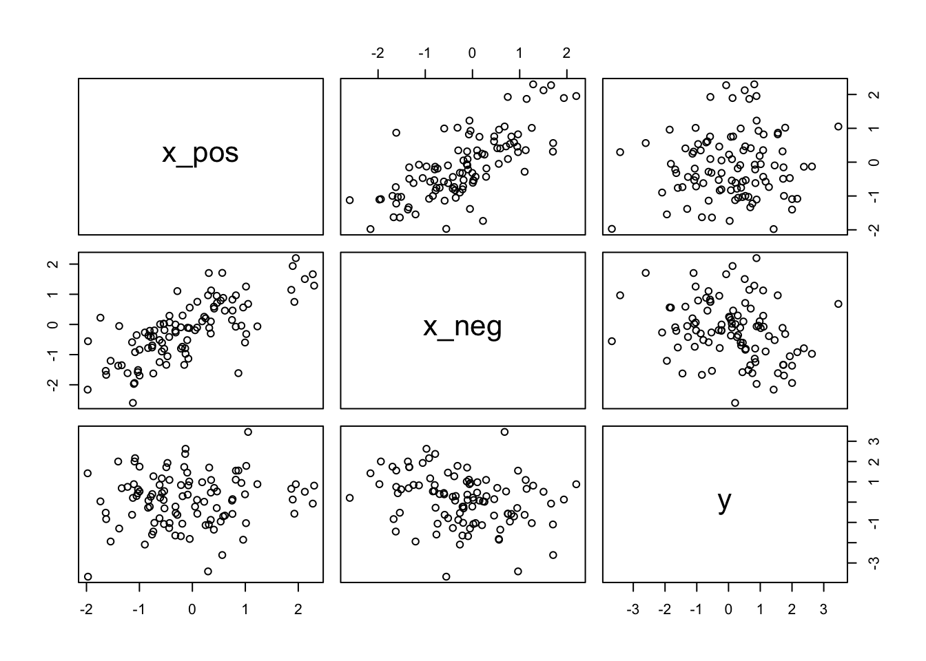
d %>%
  cor() %>%
  round(digits = 4)
## x_pos x_neg y
## x_pos 1.0000 0.7286 0.0885
## x_neg 0.7286 1.0000 -0.2673
## y 0.0885 -0.2673 1.0000m5.7a <-
brm(data = d, family = gaussian,
y ~ 1 + x_pos,
prior = c(set_prior("normal(10,100)", class = "Intercept"),
set_prior("normal(0,10)", class = "b"),
set_prior("cauchy(0,1)", class = "sigma")),
chains = 4, iter = 2000, warmup = 500, cores = 4)
p5.7a <- stanplot(m5.7a,
type = "areas",
prob = .5,
point_est = "median",
pars = "^b_") +
labs(title = "Model with x_pos") +
coord_cartesian(xlim = c(-1.5, 1.5)) +
theme_bw() +
theme(text = element_text(size = 14),
axis.ticks.y = element_blank(),
axis.text.y = element_text(hjust = 0))
m5.7b <-
brm(data = d, family = gaussian,
y ~ 1 + x_neg,
prior = c(set_prior("normal(10,100)", class = "Intercept"),
set_prior("normal(0,10)", class = "b"),
set_prior("cauchy(0,1)", class = "sigma")),
chains = 4, iter = 2000, warmup = 500, cores = 4)
p5.7b <- stanplot(m5.7b,
type = "areas",
prob = .5,
point_est = "median",
pars = "^b_") +
labs(title = "Model with x_pos") +
coord_cartesian(xlim = c(-1.5, 1.5)) +
theme_bw() +
theme(text = element_text(size = 14),
axis.ticks.y = element_blank(),
axis.text.y = element_text(hjust = 0))
m5.7c <-
brm(data = d, family = gaussian,
y ~ 1 + x_pos + x_neg,
prior = c(set_prior("normal(10,100)", class = "Intercept"),
set_prior("normal(0,10)", class = "b"),
set_prior("cauchy(0,1)", class = "sigma")),
chains = 4, iter = 2000, warmup = 500, cores = 4)
p5.7c <- stanplot(m5.7c,
type = "areas",
prob = .5,
point_est = "median",
pars = "^b_") +
labs(title = "Model with x_pos") +
coord_cartesian(xlim = c(-1.5, 1.5)) +
theme_bw() +
theme(text = element_text(size = 14),
axis.ticks.y = element_blank(),
axis.text.y = element_text(hjust = 0))
cowplot::plot_grid(p5.7a, p5.7b, p5.7c, labels = NULL, nrow = 3, align = "v")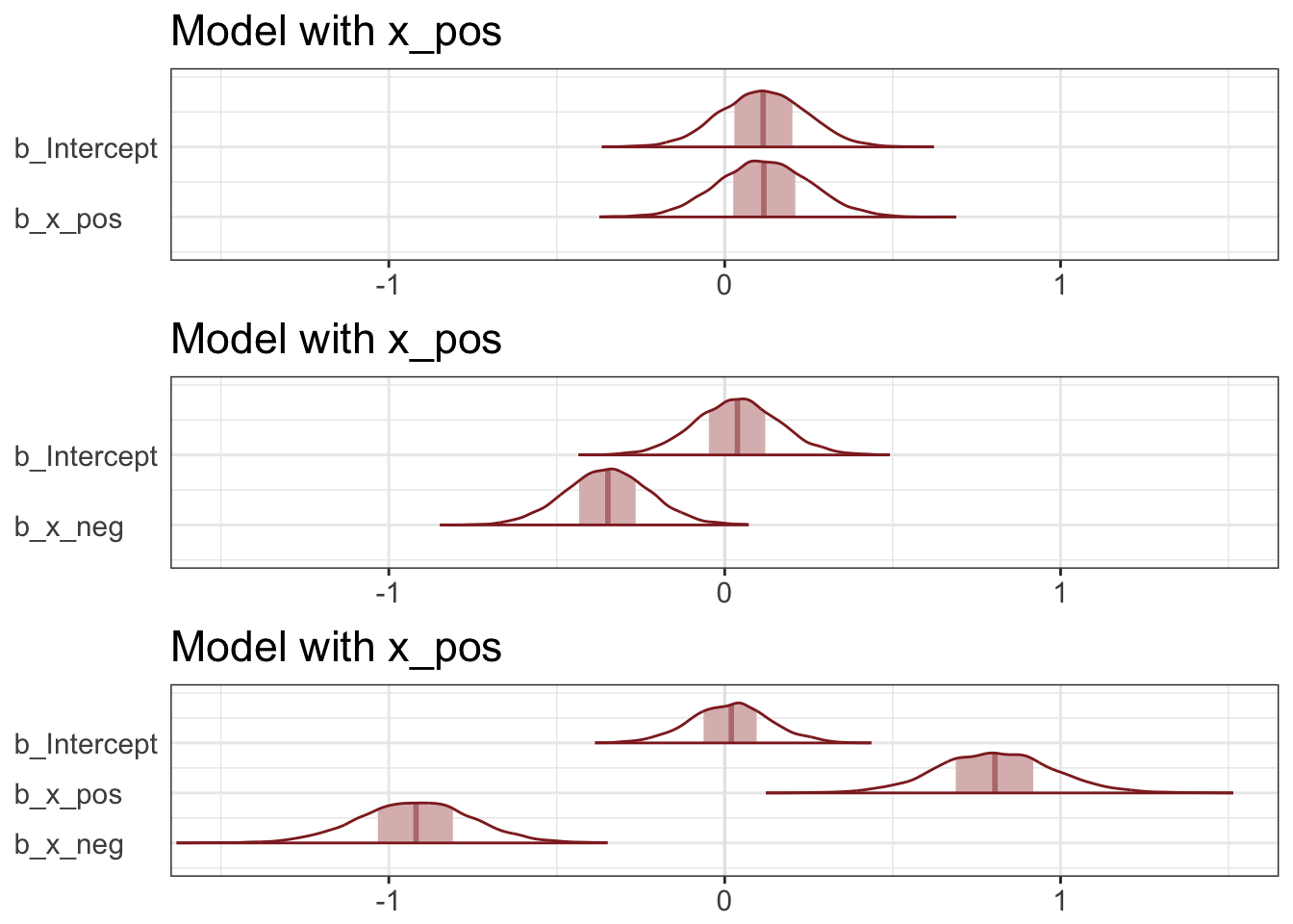
This is a context in which there are two variables correlated with the outcome, but one is positively correlated with it and the other is negatively correlated with it. In addition, both of the explanatory variables are positively correlated with one another. As a result, they tend to cancel one another out.
5.3. When adding variables hurts
Why not just fit a model that includes all predictor variables? There are several good reasons not to do so:
- Multicollinearity: when there is a very strong correlation between two or more predictor variables. The consequence of it is that the posterior distribution will say that a very large range of parameter values are plausible, from tiny associations to massive ones, even if all of the variables are in reality strongly associated with the outcome variable. This frustrating phenomenon arises from the details of how statistical control works.
- Post-treatment bias: which means statistically controlling for consequences of a causal factor.
- Overfitting
5.3.1. Multicollinear legs
N <- 100
set.seed(851)

d <-
  tibble(height    = rnorm(N, mean = 10, sd = 2),
         leg_prop  = runif(N, min = 0.4, max = 0.5),
         leg_left  = leg_prop*height + rnorm(N, mean = 0, sd = 0.02),
         leg_right = leg_prop*height + rnorm(N, mean = 0, sd = 0.02))

d %>%
  select(leg_left:leg_right) %>%
  cor() %>%
  round(digits = 4)
## leg_left leg_right
## leg_left 1.0000 0.9997
## leg_right 0.9997 1.0000Worth checking the GGally package.
library(GGally)

ggpairs(data = d, columns = c(1, 3:4))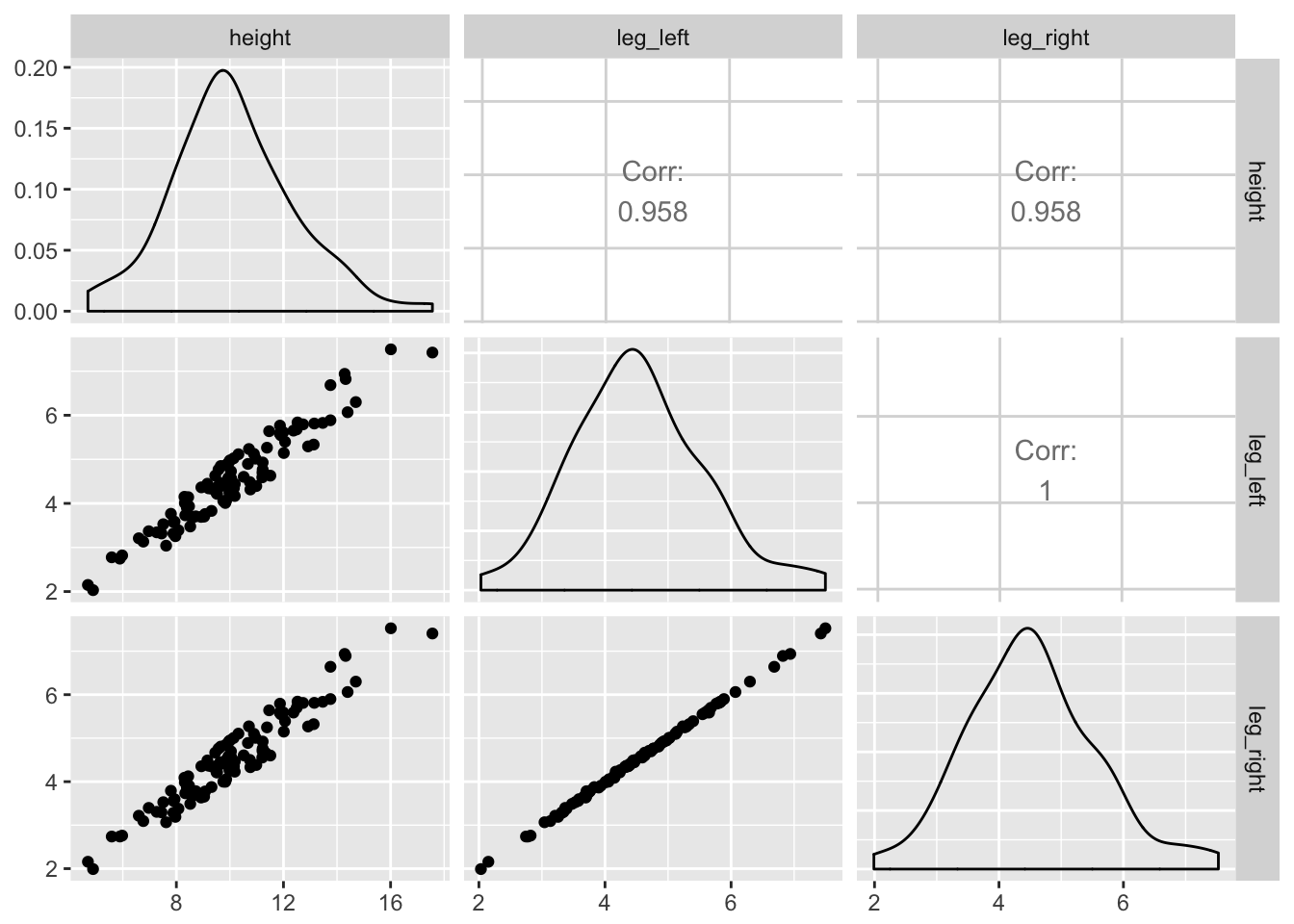
my_diag <- function(data, mapping, ...){
  pd <- ggplot(data = data, mapping = mapping) +
    geom_density(fill = "firebrick4", size = 0)
  pd
}

my_lower <- function(data, mapping, ...){
  pl <- ggplot(data = data, mapping = mapping) +
    geom_smooth(method = "lm", color = "firebrick4", size = 1/3, se = F) +
    geom_point(color = "firebrick", alpha = .8, size = 1/4)
  pl
  }

# Then plug those custom functions into ggpairs
ggpairs(data = d, columns = c(1, 3:4),
        mapping = ggplot2::aes(color = "black"),
        diag = list(continuous = my_diag),
        lower = list(continuous = my_lower)) +
  theme_bw() +
  theme(axis.text = element_blank(),
        axis.ticks = element_blank(),
        strip.background = element_rect(fill = "white"))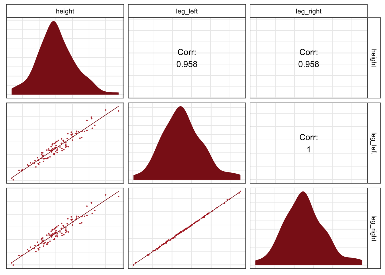
m5.8 <-
    brm(data = d, family = gaussian,
        height ~ 1 + leg_left + leg_right,
        prior = c(set_prior("normal(10,100)", class = "Intercept"),
                  set_prior("normal(2,10)", class = "b"),
                  set_prior("cauchy(0,1)", class = "sigma")),
        chains = 4, iter = 2000, warmup = 500, cores = 4)

stanplot(m5.8,
         type = "areas",
         prob = .5,
         point_est = "median") +
    labs(title = "The coefficient plot for the two-leg model",
         subtitle = "Holy smokes; look at the widths of those betas!") +
    theme_bw() +
    theme(text = element_text(size = 14),
          axis.ticks.y = element_blank(),
          axis.text.y = element_text(hjust = 0))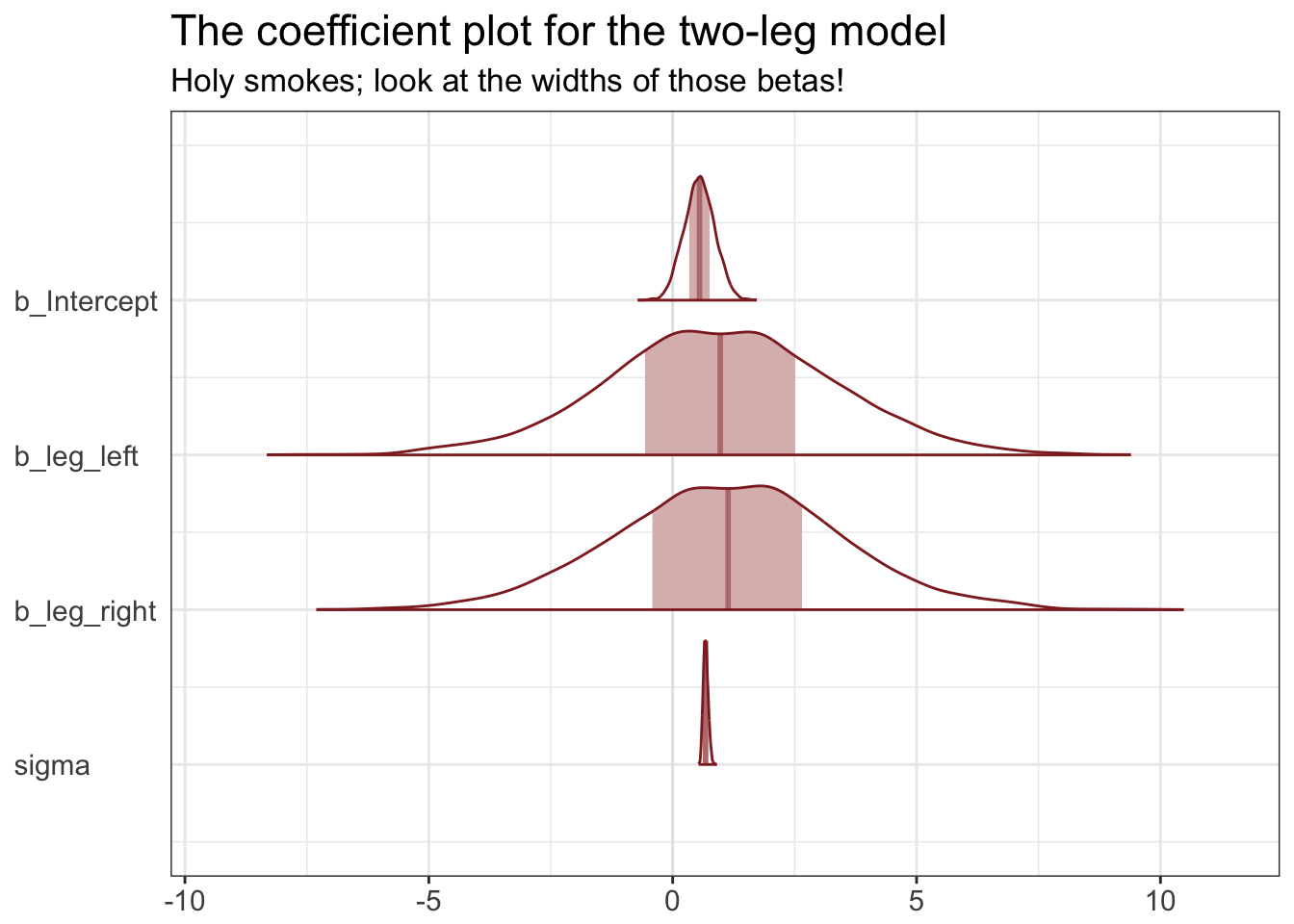
pairs(m5.8, pars = parnames(m5.8)[2:3])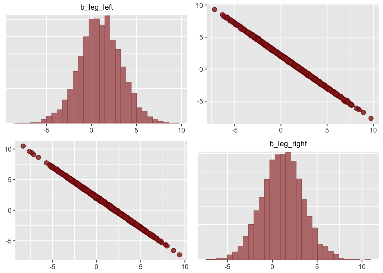
The absolute magnitude of regression slopes is not always meaningful, because the influence on prediction depends upon the product of the parameter and the data. You have to compute or plot predictions, unless you decide to standardize all of your predictors. And even then you are probably better off always plotting implied predictions than trusting your intuition.
How strong does a correlation have to get, before you should start worrying about multicollinearity? There’s no easy answer to that question. Correlations do have to get pretty high before this problem interferes with your analysis. And what matters isn’t just the correlation between a pair of variables. Rather, what matters is the correlation that remains after accounting for any other predictors.
What can be done about multicollinearity? The best thing to do is be aware of it. You can anticipate this problem by checking the predictor variables against one another in a pairs plot. Any pair or cluster of variables with very large correlations, over about 0.9, may be problematic, once included as main effects in the same model. However, it isn’t always true that highly correlated variables are completely redundant since other predictors might be correlated with only one of the pair, and so help extract the unique information each predictor provides. So you can’t know just from a table of correlations nor from a matrix of scatterplots whether multicollinearity will prevent you from including sets of variables in the same model. Still, you can usually diagnose the problem by looking for a big inflation of standard deviation, when both variables are included in the same model.
The problem of multicollinearity is really a member of a family of problems with fitting models, a family sometimes known as non-identifiability. When a parameter is non-identifiable, it means that the structure of the data and model do not make it possible to estimate the parameter’s value. Sometimes this problem arises from mistakes in coding a model, but many important types of models present non-identifiable or weakly identifiable parameters, even when coded completely correctly.
5.3.3. Post-treatment bias
Post-treatment bias arises from including variables that are consequences of other variables. This is hard to detect, even with model comparison, as post-treatment models perform well in training and testing sets.
5.4. Categorical variables
5.4.1. Binary categories
library(rethinking)
data(Howell1)
d <- Howell1

rm(Howell1)
detach(package:rethinking, unload = T)

d %>%
    glimpse()
## Observations: 544
## Variables: 4
## $ height <dbl> 151.7650, 139.7000, 136.5250, 156.8450, 145.4150, 163.8...
## $ weight <dbl> 47.82561, 36.48581, 31.86484, 53.04191, 41.27687, 62.99...
## $ age <dbl> 63.0, 63.0, 65.0, 41.0, 51.0, 35.0, 32.0, 27.0, 19.0, 5...
## $ male <int> 1, 0, 0, 1, 0, 1, 0, 1, 0, 1, 0, 1, 0, 0, 0, 1, 1, 0, 1...m5.15 <-
brm(data = d, family = gaussian,
height ~ 1 + male,
prior = c(set_prior("normal(178, 100)", class = "Intercept"),
set_prior("normal(0, 10)", class = "b"),
set_prior("cauchy(0, 2)", class = "sigma")),
chains = 4, iter = 2000, warmup = 500, cores = 4)
print(m5.15)## Family: gaussian
## Links: mu = identity; sigma = identity
## Formula: height ~ 1 + male
## Data: d (Number of observations: 544)
## Samples: 4 chains, each with iter = 2000; warmup = 500; thin = 1;
## total post-warmup samples = 6000
## ICs: LOO = NA; WAIC = NA; R2 = NA
##
## Population-Level Effects:
## Estimate Est.Error l-95% CI u-95% CI Eff.Sample Rhat
## Intercept 134.82 1.60 131.69 138.00 6000 1.00
## male 7.33 2.33 2.69 11.77 6000 1.00
##
## Family Specific Parameters:
## Estimate Est.Error l-95% CI u-95% CI Eff.Sample Rhat
## sigma 27.37 0.85 25.76 29.12 6000 1.00
##
## Samples were drawn using sampling(NUTS). For each parameter, Eff.Sample
## is a crude measure of effective sample size, and Rhat is the potential
## scale reduction factor on split chains (at convergence, Rhat = 1).The intercept is now the average height among females because when male = 0, indicating a female, the predicted mean height is just \(\alpha + \beta_m(0) = \alpha\). So the estimate says that the expected average female height is 134.85 cm. The parameter \(\beta_m\) then tells us the average difference between males and females, 7.24 cm.
Because the parameters \(\alpha\) and \(\beta_m\) are correlated with one another, you can’t just add together the boundaries to get correct boundaries for their sum.
post <-
    m5.15 %>%
    posterior_samples() %>%
    mutate(mu_male = b_Intercept + b_male) %>%
    summarise(LL = quantile(mu_male, .025) %>% round(digits = 2),
              UL = quantile(mu_male, .975) %>% round(digits = 2))

post
## LL UL
## 1 138.88 145.51The model could also be re-parameterized to include all levels of a given categorical variable:
d <-
    d %>%
    mutate(female = 1 - male)

m5.15b <-
    brm(data = d, family = gaussian,
        height ~ 0 + male + female,
        prior = c(set_prior("normal(178, 100)", class = "b"),
                  set_prior("cauchy(0, 2)", class = "sigma")),
        chains = 4, iter = 2000, warmup = 500, cores = 4)

print(m5.15b)
## Family: gaussian
## Links: mu = identity; sigma = identity
## Formula: height ~ 0 + male + female
## Data: d (Number of observations: 544)
## Samples: 4 chains, each with iter = 2000; warmup = 500; thin = 1;
## total post-warmup samples = 6000
## ICs: LOO = NA; WAIC = NA; R2 = NA
##
## Population-Level Effects:
## Estimate Est.Error l-95% CI u-95% CI Eff.Sample Rhat
## male 142.34 1.70 138.98 145.65 5736 1.00
## female 134.64 1.60 131.55 137.76 5431 1.00
##
## Family Specific Parameters:
## Estimate Est.Error l-95% CI u-95% CI Eff.Sample Rhat
## sigma 27.36 0.82 25.80 29.01 5255 1.00
##
## Samples were drawn using sampling(NUTS). For each parameter, Eff.Sample
## is a crude measure of effective sample size, and Rhat is the potential
## scale reduction factor on split chains (at convergence, Rhat = 1).With … ~ 0 + …, we tell brm() to remove the intercept.
5.4.2. Many categories
To include \(k\) categories in a linear model, you require \(k - 1\) dummy variables. Each dummy variable indicates, with the value 1, a unique category. The category with no dummy variable assigned to it ends up again as the “intercept” category.
library(rethinking)
data(milk)
d <- milk

rm(milk)
detach(package:rethinking, unload = TRUE)

library(recipes)
d2 <- recipe( ~ ., data = d) %>%
    step_dummy(clade) %>%
    prep(training = d, retain = TRUE) %>%
    juice()
m5.16 <-
brm(data = d2, family = gaussian,
kcal.per.g ~ 1 + clade_New.World.Monkey + clade_Old.World.Monkey + clade_Strepsirrhine,
prior = c(set_prior("normal(.6, 10)", class = "Intercept"),
set_prior("normal(0, 1)", class = "b"),
set_prior("cauchy(0, 2)", class = "sigma")),
chains = 4, iter = 2000, warmup = 500, cores = 4,
control = list(adapt_delta = 0.8))
m5.16 %>%
posterior_samples() %>%
mutate(mu.Ape = b_Intercept,
mu.NWM = b_Intercept + b_clade_New.World.Monkey,
mu.OWM = b_Intercept + b_clade_Old.World.Monkey,
mu.S = b_Intercept + b_clade_Strepsirrhine) %>%
select(mu.Ape:mu.S) %>%
gather(parameter) %>%
group_by(parameter) %>%
summarise(median = median(value) %>% round(digits = 2),
LL = quantile(value, probs = .025) %>% round(digits = 2),
UL = quantile(value, probs = .975) %>% round(digits = 2))## # A tibble: 4 x 4
## parameter median LL UL
## <chr> <dbl> <dbl> <dbl>
## 1 mu.Ape 0.550 0.460 0.640
## 2 mu.NWM 0.710 0.630 0.800
## 3 mu.OWM 0.790 0.680 0.900
## 4 mu.S 0.510 0.390 0.630A common error in interpretation of parameter estimates is to suppose that because one parameter is sufficiently far from zero (is “significant”) and another parameter is not (is “not significant”) that the difference between the parameters is also significant. This is not necessarily so. This isn’t just an issue for non-Bayesian analysis: if you want to know the distribution of a difference, then you must compute that difference, a contrast.
m5.16 %>%
    posterior_samples() %>%
    mutate(mu.Ape = b_Intercept,
         mu.NWM = b_Intercept + b_clade_New.World.Monkey,
         mu.OWM = b_Intercept + b_clade_Old.World.Monkey,
         mu.S   = b_Intercept + b_clade_Strepsirrhine) %>%
    mutate(dif = mu.NWM - mu.OWM) %>%
    summarise(median = median(dif) %>% round(digits = 2),
              LL = quantile(dif, probs = .025) %>% round(digits = 2),
              UL = quantile(dif, probs = .975) %>% round(digits = 2))
## median LL UL
## 1 -0.07 -0.21 0.065.4.4. Another approach: Unique intercepts
m5.16_alt <-
  brm(data = d, family = gaussian,
      kcal.per.g ~ 0 + clade,
      prior = c(set_prior("normal(.6, 10)", class = "b"),
                set_prior("cauchy(0, 2)", class = "sigma")),
      chains = 4, iter = 2000, warmup = 500, cores = 4)

print(m5.16_alt)
## Family: gaussian
## Links: mu = identity; sigma = identity
## Formula: kcal.per.g ~ 0 + clade
## Data: d (Number of observations: 29)
## Samples: 4 chains, each with iter = 2000; warmup = 500; thin = 1;
## total post-warmup samples = 6000
## ICs: LOO = NA; WAIC = NA; R2 = NA
##
## Population-Level Effects:
## Estimate Est.Error l-95% CI u-95% CI Eff.Sample Rhat
## cladeApe 0.55 0.04 0.46 0.63 6000 1.00
## cladeNewWorldMonkey 0.71 0.04 0.63 0.80 6000 1.00
## cladeOldWorldMonkey 0.79 0.05 0.68 0.90 6000 1.00
## cladeStrepsirrhine 0.51 0.06 0.39 0.62 6000 1.00
##
## Family Specific Parameters:
## Estimate Est.Error l-95% CI u-95% CI Eff.Sample Rhat
## sigma 0.13 0.02 0.10 0.18 4342 1.00
##
## Samples were drawn using sampling(NUTS). For each parameter, Eff.Sample
## is a crude measure of effective sample size, and Rhat is the potential
## scale reduction factor on split chains (at convergence, Rhat = 1).Ordinary least squares and lm
5.5.2.4. No estimate for \(\sigma\)
Using
lmwill not provide a posterior distribution for the standard deviation \(\sigma\). If you ask for a summary of the model fit,lmwill report the “residual standard error”, which is a slightly different estimate of \(\sigma\), but without any uncertainty information like a standard deviation (or standard error).
5.5.3. Building map formulas from lm formulas
The rethinking package has a convenient function that translates design formulas into map() style model formulas.
rethinking::glimmer(kcal.per.g ~ perc.fat , data = d)## alist(
## kcal_per_g ~ dnorm( mu , sigma ),
## mu <- Intercept +
## b_perc_fat*perc_fat,
## Intercept ~ dnorm(0,10),
## b_perc_fat ~ dnorm(0,10),
## sigma ~ dcauchy(0,2)
## )References
McElreath, R. (2016). Statistical rethinking: A Bayesian course with examples in R and Stan. Chapman & Hall/CRC Press.
Kurz, A. S. (2018, March 9). brms, ggplot2 and tidyverse code, by chapter. Retrieved from https://goo.gl/JbvNTj