Ockham’s razor: Models with fewer assumptions are to be preferred.
Stargazing. The most common form of model selection among practicing scientists is to search for a model in which every coefficient is statistically significant. Statisticians sometimes call this stargazing, as it is embodied by scanning for asterisks (**) trailing after estimates. The model that is full of stars, the thinking goes, is best. But such a model is not best. Whatever you think about null hypothesis significance testing in general, using it to select among structurally different models is a mistake. p-values are not designed to help you navigate between underfitting and overfitting. It is true that predictor variables that do improve prediction are not always statistically significant. It is also possible for variables that are statistically significant to do nothing useful for prediction. Since the conventional 5% threshold is purely conventional, we shouldn’t expect it to optimize anything.
6.1. The problem with parameters
Adding parameters (i.e. making the model more complex) nearly always improves the fit of a model to the data. However, while more complex models fit the data better, they often predict new data worse. But simple models, with too few parameters, tend instead to underfit, systematically overpredicting or underpredicting the data, regardless of how well future data resemble past data. So we can’t always favor either simple models or complex models.
6.1.1. More parameters always improve fit
If you adopt a model family with enough parameters, you can fit the data exactly. But such a model will make rather absurd predictions for yet-to-be-observed cases.
Model fitting can be considered a form of data compression. Parameters summarize relationships among the data. These summaries compress the data into a simpler form, although with loss of information (“lossy” compression) about the sample. The parameters can then be used to generate new data, effectively decompressing the data. However, when a model has a parameter to correspond to each datum, then there is actually no compression. The model just encodes the raw data in a different form, using parameters instead. As a result, we learn nothing about the data from such a model. Learning about the data requires using a simpler model that achieves some compression, but not too much. This view of model selection is often known as Minimum Description Length (MDL).
Overfitting produces models that fit the data extremely well, but they suffer for this within-sample accuracy by making nonsensical out-of sample predictions. An overfit model is very sensitive to the sample.
6.1.2. Too few parameters hurts, too
Underfitting produces models that are inaccurate both within and out of sample. An underfit model is insensitive to the sample.
The underfitting/overfitting dichotomy is often described as the bias-variance trade-off. “Bias” is related to underfitting, while “variance” is related to overfitting.
6.2. Information theory and model performance
In defining a target, there are two major dimensions to worry about:
- Cost-benefit analysis. How much does it cost when we’re wrong? How much do we win when we’re right?
- Accuracy in context. Some prediction tasks are inherently easier than others. So even if we ignore costs and benefits, we still need a way to judge “accuracy” that accounts for how much a model could possibly improve prediction.
What is a true model? It’s hard to define “true” probabilities, because all models are false. So what does “truth” mean in this context? It means the right probabilities, given our state of ignorance. Our state of ignorance is described by the model. The probability is in the model, not in the world. If we had all of the information relevant to producing a forecast, then rain or sun would be deterministic, and the “true” probabilities would be just 0’s and 1’s. Absent some relevant information, as in all modeling, outcomes in the small world are uncertain, even though they remain perfectly deterministic in the large world. Because of our ignorance, we can have “true” probabilities between zero and one.
6.2.2. Information and uncertainty
Information: The reduction in uncertainty derived from learning an outcome.
Information entropy: the uncertainty contained in a probability distribution is the average log probability of an event.
\[H(p) = - \text{E}\ln(p_i) = -\sum _{ i=1 }^{ n }p_i\ln(p_i)\]
L’Hôpital’s rule tells us that \(\lim _{ { p }_{ i }\rightarrow 0 }p_i\ln(p_i) = 0\).
6.2.3. From entropy to accuracy
(Kullback-Leibler or KL) Divergence: The additional uncertainty induced by using probabilities from one distribution to describe another distribution, i.e. the average difference in log probability between the target (p) and model (q). Divergence is measuring how far q is from the target p, in units of entropy.
\[D_{KL}(p,q) = \sum _{ i }p_i\left( \ln(p_i)-\ln(q_i) \right) = \sum _{ i }p_i \ln\left(\frac { p_i }{ q_i }\right) \]
Divergence depends upon direction, i.e. \(D_{KL}(p,q) \neq D_{KL}(q,p)\).
6.2.4. From divergence to deviance
To use \(D_{KL}\) to compare models, it seems like we would have to know \(p\), the target probability distribution. But there’s an amazing way out of this predicament. It helps that we are only interested in comparing the divergences of different candidates, say \(q\) and \(r\). All of this also means that all we need to know is a model’s average log-probability: \(\text{E}\ln(q_i)\) for \(q\) and \(\text{E}\ln(r_i)\) for \(r\). Neither \(\text{E}\ln(q_i)\) nor \(\text{E}\ln(r_i)\) by itself suggests a good or bad model. Only the difference \(\text{E}\ln(q_i)-\text{E}\ln(r_i)\) informs us about the divergence of each model from the target \(p\).
To approximate the relative value of \(\text{E}\ln(q_i)\), we can use a model’s deviance, which is defined as:
\[D(q) = -2\sum _{ i } \ln\left(q_i\right)\]
where \(q_i\) is just the likelihood of observation \(i\).
library(tidyverse)

d <-
    tibble(species = c("afarensis", "africanus", "habilis", "boisei",
                       "rudolfensis", "ergaster", "sapiens"),
           brain = c(438, 452, 612, 521, 752, 871, 1350),
           mass = c(37.0, 35.5, 34.5, 41.5, 55.5, 61.0, 53.5))

d <-
    d %>%
    mutate(mass.s = (mass - mean(mass))/sd(mass))

library(brms)
## Warning: package 'Rcpp' was built under R version 3.4.4# Here we specify our starting values
Inits <- list(Intercept = mean(d$brain),
mass.s = 0,
sigma = sd(d$brain))
# List of lists depending on the number of chains
InitsList <-list(Inits, Inits, Inits, Inits)
# The model
m6.8 <-
brm(data = d, family = gaussian,
brain ~ 1 + mass.s,
prior = c(set_prior("normal(0, 1000)", class = "Intercept"),
set_prior("normal(0, 1000)", class = "b"),
set_prior("cauchy(0, 10)", class = "sigma")),
chains = 4, iter = 2000, warmup = 1000, cores = 4,
inits = InitsList) # Here we put our start values in the brm() function
dfLL <-
m6.8 %>%
#log_lik() returns a matrix. Each observation gets a column and each HMC chain iteration gets a row
log_lik() %>%
as_tibble()
dfLL %>%
glimpse()## Observations: 4,000
## Variables: 7
## $ V1 <dbl> -6.595042, -6.191450, -6.496523, -6.526610, -6.635609, -6.5...
## $ V2 <dbl> -6.489443, -6.160606, -6.508486, -6.473589, -6.570281, -6.4...
## $ V3 <dbl> -6.465350, -6.573521, -6.887245, -6.651057, -6.632685, -6.6...
## $ V4 <dbl> -6.659583, -6.189061, -6.528291, -6.605774, -6.697368, -6.6...
## $ V5 <dbl> -7.041495, -6.222974, -6.978870, -7.180869, -7.085852, -7.6...
## $ V6 <dbl> -7.094083, -6.191282, -7.169668, -7.373748, -7.181638, -8.0...
## $ V7 <dbl> -7.600851, -10.666843, -7.634873, -7.390962, -7.396433, -7....dfLL <-
dfLL %>%
mutate(sums = rowSums(.),
deviance = -2*sums)quantile(dfLL$deviance, c(.025, .5, .975))## 2.5% 50% 97.5%
## 95.15443 97.50816 105.35658Since we have a posterior distribution of parameter values, there is also a posterior distribution of the deviance.
ggplot(dfLL, aes(x = deviance)) +
  theme_classic() +
  geom_density(fill = "plum", size = 0) +
  geom_vline(xintercept = quantile(dfLL$deviance, c(.025, .5, .975)),
             color = "plum4", linetype = c(2, 1, 2)) +
  scale_x_continuous(breaks = quantile(dfLL$deviance, c(.025, .5, .975)),
                     labels = c(95, 98, 105)) +
  scale_y_continuous(NULL, breaks = NULL) +
  labs(title = "The deviance distribution",
       subtitle = "The dotted lines are the 95% intervals and\nthe solid line is the median.") +
  theme(text = element_text(family = "Courier"))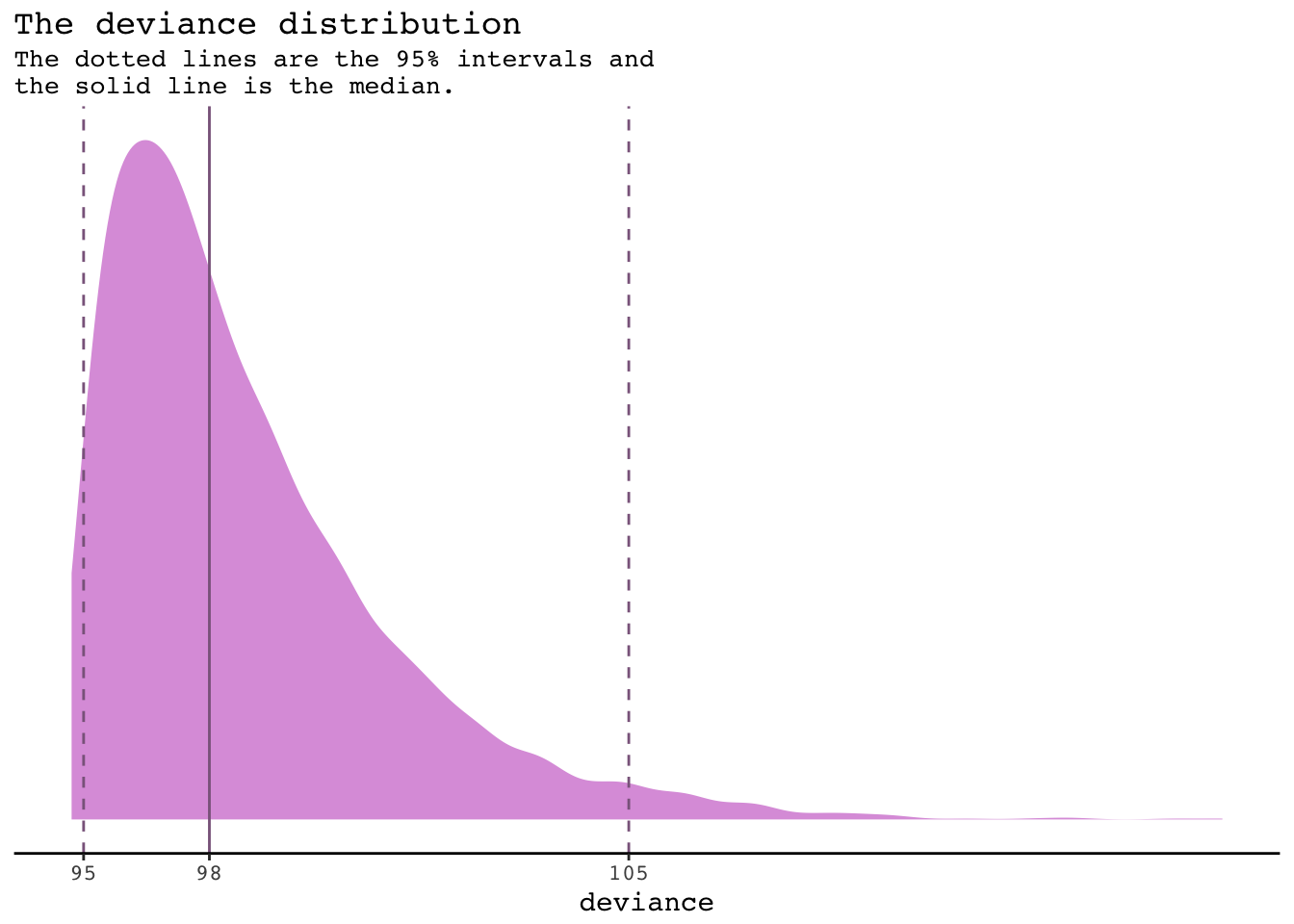
6.2.5. From deviance to out-of-sample
Deviance is an assessment of predictive accuracy, not of truth. The true model, in terms of which predictors are included, is not guaranteed to produce the best predictions. Likewise a false model, in terms of which predictors are included, is not guaranteed to produce poor predictions.
While deviance on training data always improves with additional predictor variables, deviance on future data may or may not, depending upon both the true data-generating process and how much data is available to precisely estimate the parameters. These facts form the basis for understanding both regularizing priors and information criteria.
6.3. Regularization
When the priors are flat or nearly flat, the machine interprets this to mean that every parameter value is equally plausible. As a result, the model returns a posterior that encodes as much of the training sample (as represented by the likelihood function) as possible.
A regularizing prior, when tuned properly, reduces overfitting while still allowing the model to learn the regular features of a sample. If the prior is too skeptical, however, then regular features will be missed, resulting in underfitting. So the problem is really one of tuning. Even mild skepticism can help a model do better, and doing better is all we can really hope for in the large world, where no model nor prior is optimal.
Regularizing priors are great, because they reduce overfitting. But if they are too skeptical, they prevent the model from learning from the data. So to use them most effectively, you need some way to tune them. Tuning them isn’t always easy. If you have enough data, you can split into “train” and “test” samples and then try different priors and select the one that provides the smallest deviance on the test sample. That is the essence of cross-validation, a common technique for reducing overfitting. But if you need to use all of the data to train the model, tuning the prior may not be so easy. It would be nice to have a way to predict a model’s out-of-sample deviance, to forecast its predictive accuracy, using only the sample at hand. That’s the purpose of information criteria.
Linear models in which the slope parameters use Gaussian priors, centered at zero, are sometimes known as ridge regression. Ridge regression typically takes as input a precision (\lambda) that essentially describes the narrowness of the prior. (\lambda > 0) results in less overfitting. However, just as with the Bayesian version, if (\lambda) is too large, we risk underfitting.
6.4. Information criteria
The phenomenon behind information criteria is that it is possible to trace the average out-of-sample deviance for each model.
Information criteria are not consistent for model identification. These criteria aim to nominate the model that will produce the best predictions, as judged by out-of-sample deviance.
6.4.1. Deviance Information Criterion (DIC)
DIC is essentially a version of AIC that is aware of informative priors. Like AIC, it assumes a multivariate Gaussian posterior distribution. DIC is calculated from the posterior distribution of the training deviance.
If any parameter in the posterior is substantially skewed, and also has a substantial effect on prediction, then DIC like AIC can go horribly wrong.
DIC is calculated as:
\[\text{DIC}=\bar { D } +\left( \bar { D } -\hat { D } \right) =\bar { D } -{ p }_{ D }\]
where \(D\) is the posterior distribution of deviance, \(\bar{D}\) indicates the average of \(D\), and \(\hat{D}\) is the deviance calculated at the posterior mean. The difference \(\bar { D } -\hat { D } = { p }_{ D }\) is analogous to the number of parameters used in computing AIC. It is an “effective” number of parameters that measures how flexible the model is in fitting the training sample.
The \(p_D\) term is sometimes called a penalty term. It is just the expected distance between the deviance in-sample and the deviance out-of-sample. In the case of flat priors, DIC reduces directly to AIC, because the expected distance is just the number of parameters. But more generally, \(p_D\) will be some fraction of the number of parameters, because regularizing priors constrain a model’s flexibility.
6.4.2 Widely Applicable Information Criterion (WAIC)
WAIC is just an estimate of out-of-sample deviance. It does not require a multivariate Gaussian posterior, and it is often more accurate than DIC. The distinguishing feature of WAIC is that it is pointwise. This means that uncertainty in prediction is considered case-by-case, or point-by-point, in the data.
Define \(\Pr(y_i)\) as the average likelihood of observation \(i\) in the training sample. This means we compute the likelihood of \(y_i\) for each set of parameters sampled from the posterior distribution. Then we average the likelihoods for each observation \(i\) and finally sum over all observations. This produces the first part of WAIC, the log-pointwise-predictive-density, lppd:
\[\text{lppd} = \sum _{ i } ^{N} \ln \Pr\left(y_i\right)\]
The lppd is just a pointwise analog of deviance, averaged over the posterior distribution. If you multiplied it by -2, it’d be similar to the deviance.
Define \(V(y_i)\) as the variance in log-likelihood for observation \(i\) in the training sample. This means we compute the log-likelihood of \(y_i\) for each sample from the posterior distribution. Then we take the variance of those values. Then the effective number of parameters \(p_{WAIC}\) is defined as:
\[p_{WAIC} = \sum _{ i } ^{N} V\left(y_i\right)\]
WAIC is defined as:
\[\text{WAIC} = -2\left( \text{lppd} - p_{WAIC} \right)\]
waic(m6.8)## WAIC SE
## 102.13 6.27Because WAIC requires splitting up the data into independent observations, it is sometimes hard to define. In time series, you can compute WAIC as if each observation were independent of the others, but it’s not clear what the resulting value means.
A more general issue with all of these predictive information criteria: their validity depends upon the predictive task at hand.
6.5. Using information criteria
Frequently, people discuss model selection, which usually means choosing the model with the lowest AIC/DIC/WAIC value and then discarding the others. But this kind of selection procedure discards the information about relative model accuracy contained in the differences among the AIC/DIC/WAIC values. This information is useful because sometimes the differences are large and sometimes they are small. Just as relative posterior probability provides advice about how confident we might be about parameters (conditional on the model), relative model accuracy provides advice about how confident we might be about models (conditional on the set of models compared).
6.5.1. Model comparison
Model comparison means using DIC/WAIC in combination with the estimates and posterior predictive checks from each model. It is just as important to understand why a model outperforms another as it is to measure the performance difference.
Compared models must be fit to exactly the same observations. A model fit to fewer observations will almost always have a better deviance and AIC/DIC/WAIC value, because it has been asked to predict less.
library(rethinking)

data(milk)
d <-
  milk %>%
  filter(complete.cases(.))
rm(milk)

d <-
  d %>%
  mutate(neocortex = neocortex.perc/100)

detach(package:rethinking, unload = T)

# Model with no predictors (just the intercept)
Inits <- list(Intercept = mean(d$kcal.per.g),
              sigma = sd(d$kcal.per.g))
InitsList <-list(Inits, Inits, Inits, Inits)
m6.11 <-
    brm(data = d, family = gaussian,
        kcal.per.g ~ 1,
        prior = c(set_prior("uniform(-1000, 1000)", class = "Intercept"),
                  set_prior("uniform(0, 100)", class = "sigma")),
        chains = 4, iter = 2000, warmup = 1000, cores = 4,
        inits = InitsList)
## Warning: It appears as if you have specified an upper bounded prior on a parameter that has no natural upper bound.
## If this is really what you want, please specify argument 'ub' of 'set_prior' appropriately.
## Warning occurred for prior
## sigma ~ uniform(0, 100)# Model with only neocortex
Inits <- list(Intercept = mean(d$kcal.per.g),
neocortex = 0,
sigma = sd(d$kcal.per.g))
InitsList <-list(Inits, Inits, Inits, Inits)
m6.12 <-
brm(data = d, family = gaussian,
kcal.per.g ~ 1 + neocortex,
prior = c(set_prior("uniform(-1000, 1000)", class = "Intercept"),
set_prior("uniform(-1000, 1000)", class = "b"),
set_prior("uniform(0, 100)", class = "sigma")),
chains = 4, iter = 2000, warmup = 1000, cores = 4,
inits = InitsList)## Warning: It appears as if you have specified a lower bounded prior on a parameter that has no natural lower bound.
## If this is really what you want, please specify argument 'lb' of 'set_prior' appropriately.
## Warning occurred for prior
## b ~ uniform(-1000, 1000)## Warning: It appears as if you have specified an upper bounded prior on a parameter that has no natural upper bound.
## If this is really what you want, please specify argument 'ub' of 'set_prior' appropriately.
## Warning occurred for prior
## b ~ uniform(-1000, 1000)
## sigma ~ uniform(0, 100)# Model with only log mass
Inits <- list(Intercept = mean(d$kcal.per.g),
`log(mass)` = 0,
sigma = sd(d$kcal.per.g))
InitsList <-list(Inits, Inits, Inits, Inits)
m6.13 <- brm(data = d, family = gaussian,
kcal.per.g ~ 1 + log(mass),
prior = c(set_prior("uniform(-1000, 1000)", class = "Intercept"),
set_prior("uniform(-1000, 1000)", class = "b"),
set_prior("uniform(0, 100)", class = "sigma")),
chains = 4, iter = 2000, warmup = 1000, cores = 4,
inits = InitsList)## Warning: It appears as if you have specified a lower bounded prior on a parameter that has no natural lower bound.
## If this is really what you want, please specify argument 'lb' of 'set_prior' appropriately.
## Warning occurred for prior
## b ~ uniform(-1000, 1000)
## Warning: It appears as if you have specified an upper bounded prior on a parameter that has no natural upper bound.
## If this is really what you want, please specify argument 'ub' of 'set_prior' appropriately.
## Warning occurred for prior
## b ~ uniform(-1000, 1000)
## sigma ~ uniform(0, 100)
# Model with both neocortex and log mass
Inits <- list(Intercept = mean(d$kcal.per.g),
neocortex = 0,
`log(mass)` = 0,
sigma = sd(d$kcal.per.g))
InitsList <-list(Inits, Inits, Inits, Inits)
m6.14 <-
brm(data = d, family = gaussian,
kcal.per.g ~ 1 + neocortex + log(mass),
prior = c(set_prior("uniform(-1000, 1000)", class = "Intercept"),
set_prior("uniform(-1000, 1000)", class = "b"),
set_prior("uniform(0, 100)", class = "sigma")),
chains = 4, iter = 2000, warmup = 1000, cores = 4,
inits = InitsList)## Warning: It appears as if you have specified a lower bounded prior on a parameter that has no natural lower bound.
## If this is really what you want, please specify argument 'lb' of 'set_prior' appropriately.
## Warning occurred for prior
## b ~ uniform(-1000, 1000)
## Warning: It appears as if you have specified an upper bounded prior on a parameter that has no natural upper bound.
## If this is really what you want, please specify argument 'ub' of 'set_prior' appropriately.
## Warning occurred for prior
## b ~ uniform(-1000, 1000)
## sigma ~ uniform(0, 100)6.5.1.1. Comparing WAIC values
One way to compare models is using the waic function:
waic(m6.11, m6.12, m6.13, m6.14)## WAIC SE
## m6.11 -8.80 3.74
## m6.12 -7.33 3.22
## m6.13 -8.79 4.14
## m6.14 -17.07 5.08
## m6.11 - m6.12 -1.46 1.22
## m6.11 - m6.13 -0.01 2.28
## m6.11 - m6.14 8.27 4.85
## m6.12 - m6.13 1.45 2.96
## m6.12 - m6.14 9.73 4.96
## m6.13 - m6.14 8.28 3.44Alternatively, first compute the WAIC for each model and use the compare_ic function:
w.m6.11 <- waic(m6.11)
w.m6.12 <- waic(m6.12)
w.m6.13 <- waic(m6.13)
w.m6.14 <- waic(m6.14)

compare_ic(w.m6.11, w.m6.12, w.m6.13, w.m6.14)
## WAIC SE
## m6.11 -8.80 3.74
## m6.12 -7.33 3.22
## m6.13 -8.79 4.14
## m6.14 -17.07 5.08
## m6.11 - m6.12 -1.46 1.22
## m6.11 - m6.13 -0.01 2.28
## m6.11 - m6.14 8.27 4.85
## m6.12 - m6.13 1.45 2.96
## m6.12 - m6.14 9.73 4.96
## m6.13 - m6.14 8.28 3.44tibble(model = c("m6.11", "m6.12", "m6.13", "m6.14"),
waic = c(w.m6.11$waic, w.m6.12$waic, w.m6.13$waic, w.m6.14$waic),
se = c(w.m6.11$se_waic, w.m6.12$se_waic, w.m6.13$se_waic, w.m6.14$se_waic)) %>%
ggplot() +
theme_classic() +
geom_pointrange(aes(x = model, y = waic,
ymin = waic - se,
ymax = waic + se),
shape = 21, color = "plum4", fill = "plum") +
coord_flip() +
labs(x = NULL, y = NULL,
title = "My custom WAIC plot") +
theme(text = element_text(family = "Courier"),
axis.ticks.y = element_blank())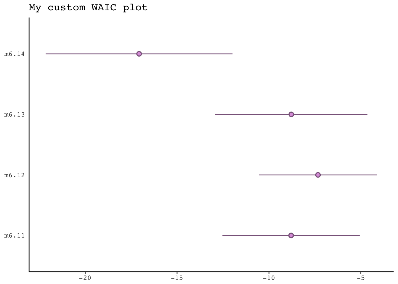
Worth checking the LOO information criteria.
I replicated the compare function from the rethinking package. It returns a table in which models are ranked from best to worst, with six columns of information:
- WAIC is the WAIC for each model. Smaller WAIC indicates better estimated out-of-sample deviance.
- pWAIC is the estimated effective number of parameters. This provides a clue as to how flexible each model is in fitting the sample.
- dWAIC is the difference between each WAIC and the lowest WAIC. Since only relative deviance matters, this column shows the differences in relative fashion.
- weight is the Akaike weight for each model. These values are transformed information criterion values.
- SE is the standard error of the WAIC estimate. WAIC is an estimate, and provided the sample size N is large enough, its uncertainty will be well approximated by its standard error. So this SE value isn’t necessarily very precise, but it does provide a check against overconfidence in differences between WAIC values.
- dSE is the standard error of the difference in WAIC between each model and the top-ranked model. So it is missing for the top model.
# ... are the fitted models
compare_waic <- function (..., sort = "WAIC", func = "WAIC")
{
    mnames <- as.list(substitute(list(...)))[-1L]

    L <- list(...)
    if (is.list(L[[1]]) && length(L) == 1) {L <- L[[1]]}

    classes <- as.character(sapply(L, class))
    if (any(classes != classes[1])) {
        warning("Not all model fits of same class.\nThis is usually a bad idea, because it implies they were fit by different algorithms.\nCheck yourself, before you wreck yourself.")
    }

    nobs_list <- try(sapply(L, nobs))
    if (any(nobs_list != nobs_list[1])) {
        nobs_out <- paste(mnames, nobs_list, "\n")
        nobs_out <- concat(nobs_out)
        warning(concat("Different numbers of observations found for at least two models.\nInformation criteria only valid for comparing models fit to exactly same observations.\nNumber of observations for each model:\n",
                       nobs_out))
    }

    dSE.matrix <- matrix(NA, nrow = length(L), ncol = length(L))

    if (func == "WAIC") {
        WAIC.list <- lapply(L, function(z) WAIC(z, pointwise = TRUE))
        p.list <- sapply(WAIC.list, function(x) x$p_waic)
        se.list <- sapply(WAIC.list, function(x) x$se_waic)
        IC.list <- sapply(WAIC.list, function(x) x$waic)
        #mnames <- sapply(WAIC.list, function(x) x$model_name)
        colnames(dSE.matrix) <- mnames
        rownames(dSE.matrix) <- mnames
        for (i in 1:(length(L) - 1)) {
            for (j in (i + 1):length(L)) {
                waic_ptw1 <- WAIC.list[[i]]$pointwise[ , 3]
                waic_ptw2 <- WAIC.list[[j]]$pointwise[ , 3]
                dSE.matrix[i, j] <- as.numeric(sqrt(length(waic_ptw1) *
                                                        var(waic_ptw1 - waic_ptw2)))
                dSE.matrix[j, i] <- dSE.matrix[i, j]
            }
        }
    }

    #if (!(the_func %in% c("DIC", "WAIC", "LOO"))) {
    #    IC.list <- lapply(L, function(z) func(z))
    #}
    IC.list <- unlist(IC.list)
    dIC <- IC.list - min(IC.list)
    w.IC <- rethinking::ICweights(IC.list)
    if (func == "WAIC") {
        topm <- which(dIC == 0)
        dSEcol <- dSE.matrix[, topm]
        result <- data.frame(WAIC = IC.list, pWAIC = p.list,
                             dWAIC = dIC, weight = w.IC, SE = se.list, dSE = dSEcol)
    }

    #if (!(the_func %in% c("DIC", "WAIC", "LOO"))) {
    #    result <- data.frame(IC = IC.list, dIC = dIC, weight = w.IC)
    #}
    rownames(result) <- mnames
    if (!is.null(sort)) {
        if (sort != FALSE) {
            if (sort == "WAIC")
                sort <- func
            result <- result[order(result[[sort]]), ]
        }
    }
    new("compareIC", output = result, dSE = dSE.matrix)
}

compare_waic(m6.11, m6.12, m6.13, m6.14)
## WAIC pWAIC dWAIC weight SE dSE
## m6.14 -17.1 3.0 0.0 0.96 5.08 NA
## m6.11 -8.8 1.3 8.3 0.02 3.74 4.85
## m6.13 -8.8 2.0 8.3 0.02 4.14 3.44
## m6.12 -7.3 1.9 9.7 0.01 3.22 4.96Akaike weights help by rescaling. The weight for a model \(i\) in a set of \(m\) models is given by:
\[w_i = \frac {\exp \left( -\frac { 1 }{ 2 } \text{dWAIC}_i \right)} {\sum _{j=1}^{m}{\exp \left( -\frac { 1 }{ 2 } \text{dWAIC}_j \right)} }\] where \(\text{dWAIC}_j\) is the same as dWAIC from the compare table output.
A model’s weight is an estimate of the probability that the model will make the best predictions on new data, conditional on the set of models considered.
WAIC as the expected deviance of a model on future data. That is to say that WAIC gives us an estimate of \(\text{E}(D_{\text{test}})\). Akaike weights convert these deviance values, which are log-likelihoods, to plain likelihoods and then standardize them all.
The Akaike weights are analogous to posterior probabilities of models, conditional on expected future data. However, given all the strong assumptions about repeat sampling that go into calculating WAIC, you can’t take this heuristic too seriously. The future is unlikely to be exactly like the past, after all.
6.5.1.2. Comparing estimates
Comparing estimates helps in at least two major ways. First, it is useful to understand why a particular model or models have lower WAIC values. Changes in posterior distributions, across models, provide useful hints. Second, regardless of WAIC values, we often want to know whether some parameter’s posterior distribution is stable across models.
library(broom)

my_coef_tab <-
  rbind(tidy(m6.11), tidy(m6.12), tidy(m6.13), tidy(m6.14)) %>%
  mutate(model = c(rep("m6.11", times = nrow(tidy(m6.11))),
                   rep("m6.12", times = nrow(tidy(m6.12))),
                   rep("m6.13", times = nrow(tidy(m6.13))),
                   rep("m6.14", times = nrow(tidy(m6.14))))
         ) %>%
  filter(term != "lp__") %>%
  select(model, everything()) %>%
  complete(term = distinct(., term), model) %>%
  rbind(
     tibble(
       model = NA,
       term = c("b_logmass", "b_neocortex", "sigma", "b_Intercept"),
       estimate = NA,
       std.error = NA,
       lower = NA,
       upper = NA)) %>%
  mutate(axis = ifelse(is.na(model), term, model),
         model = factor(model, levels = c("m6.11", "m6.12", "m6.13", "m6.14")),
         term = factor(term, levels = c("b_logmass", "b_neocortex", "sigma", "b_Intercept", NA))) %>%
  arrange(term, model) %>%
  mutate(axis_order = letters[1:20],
         axis = ifelse(str_detect(axis, "m6."), str_c("      ", axis), axis))

ggplot(data = my_coef_tab,
       aes(x = axis_order,
           y = estimate,
           ymin = lower,
           ymax = upper)) +
  theme_classic() +
  geom_hline(yintercept = 0, color = "plum4", alpha = 1/8) +
  geom_pointrange(shape = 21, color = "plum4", fill = "plum") +
  scale_x_discrete(NULL, labels = my_coef_tab$axis) +
  ggtitle("My coeftab() plot") +
  coord_flip() +
  theme(panel.grid = element_blank(),
        axis.ticks.y = element_blank(),
        axis.text.y = element_text(hjust = 0))
## Warning: Removed 8 rows containing missing values (geom_pointrange).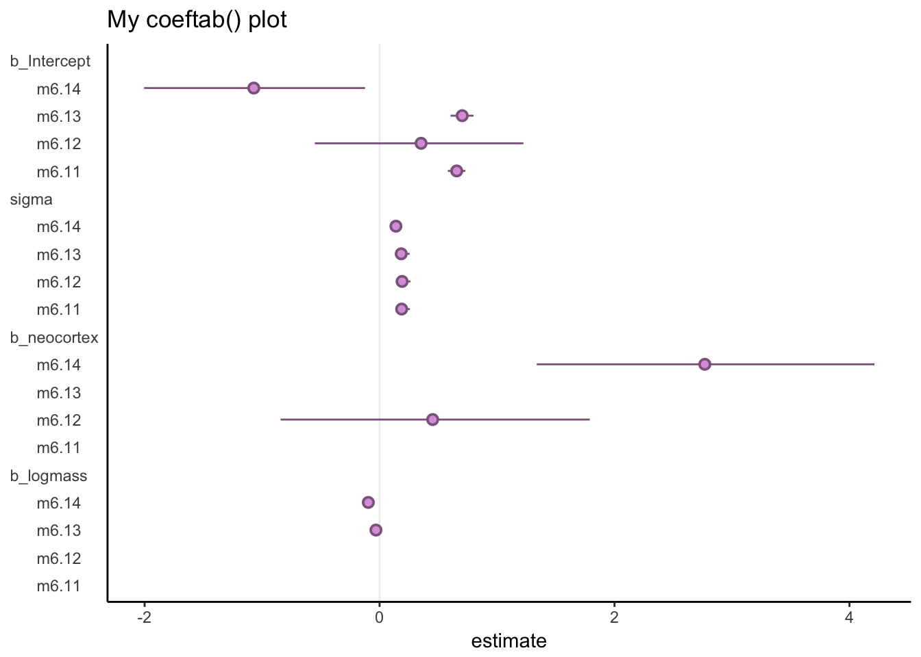
6.5.2. Model averaging
Model averaging means using DIC/WAIC to construct a posterior predictive distribution that exploits what we know about relative accuracy of the models. This helps guard against overconfidence in model structure, in the same way that using the entire posterior distribution helps guard against overconfidence in parameter values.
nd <-
    tibble(neocortex = seq(from = .5, to = .8, length.out = 30),
           mass = rep(4.5, times = 30))

ftd <-
    fitted(m6.14, newdata = nd) %>%
    as_tibble() %>%
    bind_cols(nd)

pp_average(m6.11, m6.12, m6.13, m6.14,
           weights = "waic",
           method = "fitted",  # for new data predictions, use method = "predict"
           newdata = nd) %>%
  as_tibble() %>%
  bind_cols(nd) %>%

  ggplot(aes(x = neocortex, y = Estimate)) +
  theme_classic() +
  geom_ribbon(aes(ymin = `2.5%ile`, ymax = `97.5%ile`),
              fill = "plum", alpha = 1/3) +
  geom_line(color = "plum2") +
  geom_ribbon(data = ftd, aes(ymin = `2.5%ile`, ymax = `97.5%ile`),
              fill = "transparent", color = "plum3", linetype = 2) +
  geom_line(data = ftd,
              color = "plum3", linetype = 2) +
  geom_point(data = d, aes(x = neocortex, y = kcal.per.g),
             size = 2, color = "plum4") +
  labs(y = "kcal.per.g") +
  coord_cartesian(xlim = range(d$neocortex),
                  ylim = range(d$kcal.per.g))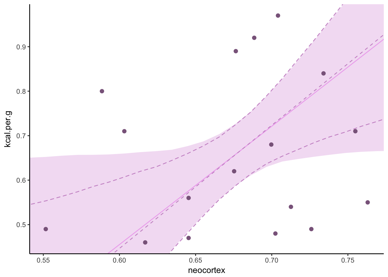
Model averaging will never make a predictor variable appear more influential than it already appears in any single model.
Bonus: \(R^2\) revisited
The usual definition of \(R^2\) has a problem for Bayesian fits. Check the paper by Gelman, Goodrich, Gabry, and Ali.
bayes_R2(m6.14) %>% round(digits = 3)## Estimate Est.Error 2.5%ile 97.5%ile
## R2 0.497 0.128 0.172 0.664rbind(bayes_R2(m6.11),
bayes_R2(m6.12),
bayes_R2(m6.13),
bayes_R2(m6.14)) %>%
as_tibble() %>%
mutate(model = c("m6.11", "m6.12", "m6.13", "m6.14"),
r_square_posterior_mean = round(Estimate, digits = 2)) %>%
select(model, r_square_posterior_mean)## # A tibble: 4 x 2
## model r_square_posterior_mean
## <chr> <dbl>
## 1 m6.11 0.
## 2 m6.12 0.0700
## 3 m6.13 0.150
## 4 m6.14 0.500# model b6.13
m6.13.R2 <-
bayes_R2(m6.13, summary = F) %>%
as_tibble() %>%
rename(R2.13 = R2)
# model b6.14
m6.14.R2 <-
bayes_R2(m6.14, summary = F) %>%
as_tibble() %>%
rename(R2.14 = R2)
# Let's put them in the same data object
combined_R2s <-
bind_cols(m6.13.R2, m6.14.R2) %>%
mutate(dif = R2.14 - R2.13)
# A simple density plot
combined_R2s %>%
ggplot(aes(x = R2.13)) +
theme_classic() +
geom_density(size = 0, fill = "springgreen4", alpha = 2/3) +
geom_density(aes(x = R2.14),
size = 0, fill = "springgreen3", alpha = 2/3) +
scale_y_continuous(NULL, breaks = NULL) +
coord_cartesian(xlim = 0:1) +
labs(x = NULL,
title = expression(paste(italic("R")^{2}, " distributions")),
subtitle = "Going from left to right, these are for\nmodels m6.13 and m6.14.")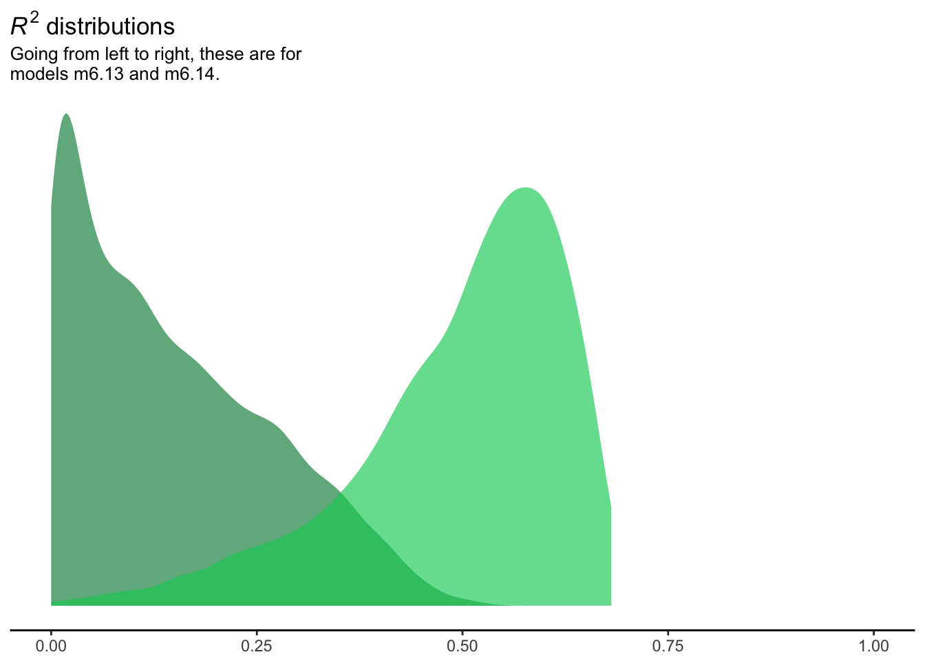
combined_R2s %>%
  ggplot(aes(x = dif)) +
  theme_classic() +
  geom_density(size = 0, fill = "springgreen") +
  geom_vline(xintercept = quantile(combined_R2s$dif,
                                   probs = c(.025, .5, .975)),
             color = "white", size = c(1/2, 1, 1/2)) +
  scale_y_continuous(NULL, breaks = NULL) +
  labs(x = expression(paste(Delta, italic("R")^{2})),
       subtitle = "This is how much more variance, in terms\nof %, model b6.14 explained compared to\nmodel b6.13. The white lines are the\nposterior median and 95% percentiles.")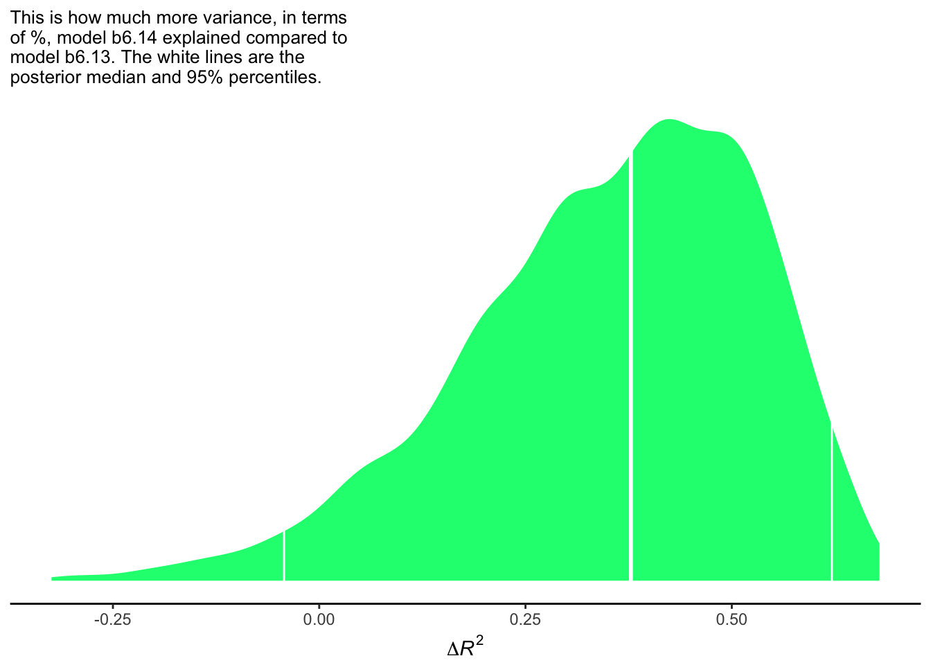
References
McElreath, R. (2016). Statistical rethinking: A Bayesian course with examples in R and Stan. Chapman & Hall/CRC Press.
Kurz, A. S. (2018, March 9). brms, ggplot2 and tidyverse code, by chapter. Retrieved from https://goo.gl/JbvNTj