Conditioning is one of the most important principles of statistical inference. Posterior distributions are conditional on the data. All model-based inference is conditional on the model.
To model deeper conditionality, where the importance of one predictor depends upon another predictor, we need interaction. Interaction is a kind of conditioning, a way of allowing parameters (really their posterior distributions) to be conditional on further aspects of the data.
7.1. Building an interaction
library(rethinking)
data(rugged)
d <- rugged

detach(package:rethinking, unload = T)
library(brms)
## Warning: package 'brms' was built under R version 3.4.4## Warning: package 'Rcpp' was built under R version 3.4.4rm(rugged)
library(tidyverse)
# make log version of outcome
d <-
d %>%
mutate(log_gdp = log(rgdppc_2000))
# extract countries with GDP data
dd <-
d %>%
filter(complete.cases(rgdppc_2000))
# split countries into Africa and not-Africa
d.A1 <-
dd %>%
filter(cont_africa == 1)
d.A0 <-
dd %>%
filter(cont_africa == 0)m7.1 <-
brm(data = d.A1, family = gaussian,
log_gdp ~ 1 + rugged,
prior = c(set_prior("normal(8, 100)", class = "Intercept"),
set_prior("normal(0, 1)", class = "b"),
set_prior("cauchy(0, 1)", class = "sigma")),
chains = 4, iter = 2000, warmup = 1000, cores = 4)
m7.2 <-
brm(data = d.A0, family = gaussian,
log_gdp ~ 1 + rugged,
prior = c(set_prior("normal(8, 100)", class = "Intercept"),
set_prior("normal(0, 1)", class = "b"),
set_prior("cauchy(0, 1)", class = "sigma")),
chains = 4, iter = 2000, warmup = 1000, cores = 4)nd <-
tibble(rugged = seq(from = 0,
to = 6.3,
length.out = 30))
fit.7.1 <-
fitted(m7.1, newdata = nd) %>%
as_tibble() %>%
bind_cols(nd)
fit.7.2 <-
fitted(m7.2, newdata = nd) %>%
as_tibble() %>%
bind_cols(nd)
# Here we'll put both in a single data object, with fit.7.1 stacked atop fit.7.2
fit.both <-
bind_rows(fit.7.1, fit.7.2) %>%
mutate(cont_africa = rep(c("Africa", "not Africa"), each = 30))
library(ggthemes)
dd %>%
mutate(cont_africa = ifelse(cont_africa == 1, "Africa", "not Africa")) %>%
ggplot(aes(x = rugged)) +
theme_pander() +
scale_colour_pander() +
scale_fill_pander() +
geom_ribbon(data = fit.both,
aes(ymin = `2.5%ile`,
ymax = `97.5%ile`,
fill = cont_africa),
alpha = 1/4) +
geom_line(data = fit.both,
aes(y = Estimate,
color = cont_africa)) +
geom_point(aes(y = log_gdp, color = cont_africa),
size = 2/3) +
scale_x_continuous(expand = c(0, 0)) +
labs(x = "Terrain Ruggedness Index",
y = "log GDP from year 2000") +
facet_wrap(~cont_africa) +
theme(text = element_text(family = "Times"),
legend.position = "none")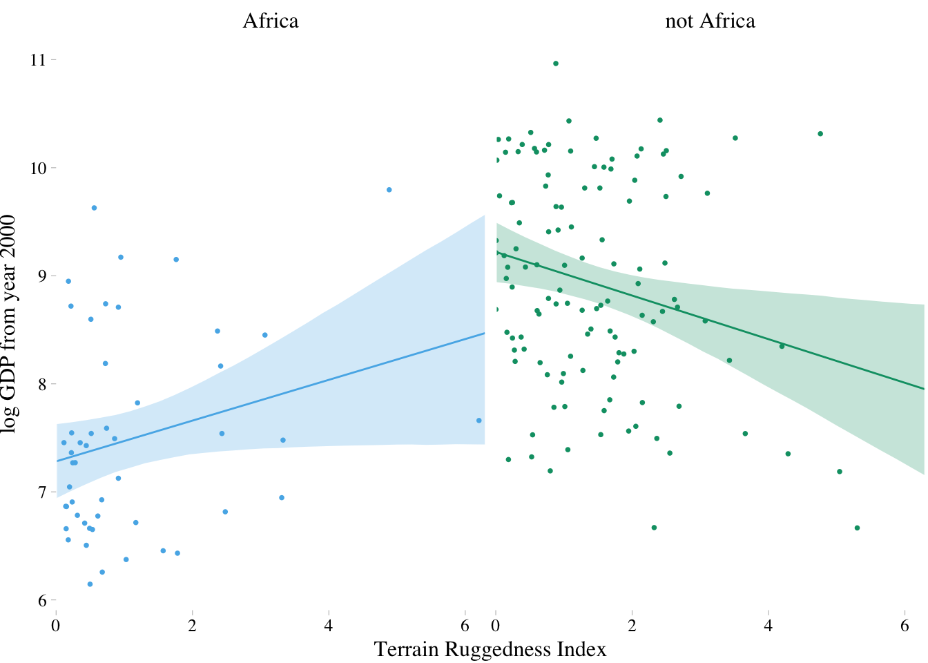
150+ color palettes by Canva derived from photos and impactful websites.
There are some reasons for why it is not a good idea to split the data as above:
- First, there are usually some parameters, such as \(\sigma\), that the model says do not depend in any way upon an African identity for each nation. By splitting the data table, you are hurting the accuracy of the estimates for these parameters, because you are essentially making two less-accurate estimates instead of pooling all of the evidence into one estimate. In effect, you have accidentally assumed that variance differs between African and non-African nations. There’s nothing wrong with that sort of assumption. But you want to avoid accidental assumptions.
- Second, in order to acquire probability statements about the variable you used to split the data,
cont_africain this case, you need to include it in the model. Otherwise, you have only the weakest sort of statistical argument.- Third, we may want to use information criteria or another method to compare models. For this, we need models that use all of the same data. This means we can’t split the data, but have to make the model split the data.
- There are advantages to borrowing information across categories. This is especially true when sample sizes vary across categories, such that overfitting risk is higher within some categories. Multilevel models borrow information in this way, in order to improve estimates in all categories.
7.1.1. Adding a dummy variable doesn’t work
The model to fit here is:
\[\begin{eqnarray} { Y }_{ i } & \sim & Normal({ \mu }_{ i },\sigma ) & \text{<- likelihood } \\ { \mu }_{ i } & = & \alpha +\beta_R { R }_{ i } +\beta_A { A }_{ i } & \text{<- linear model} \end{eqnarray}\]
m7.3 <-
  brm(data = dd, family = gaussian,
      log_gdp ~ 1 + rugged,
      prior = c(set_prior("normal(8, 100)", class = "Intercept"),
                set_prior("normal(0, 1)", class = "b"),
                set_prior("uniform(0, 10)", class = "sigma")),
      chains = 4, iter = 2000, warmup = 1000, cores = 4)
## Warning: It appears as if you have specified an upper bounded prior on a parameter that has no natural upper bound.
## If this is really what you want, please specify argument 'ub' of 'set_prior' appropriately.
## Warning occurred for prior
## sigma ~ uniform(0, 10)m7.4 <-
brm(data = dd, family = gaussian,
log_gdp ~ 1 + rugged + cont_africa,
prior = c(set_prior("normal(8, 100)", class = "Intercept"),
set_prior("normal(0, 1)", class = "b"),
set_prior("uniform(0, 10)", class = "sigma")),
chains = 4, iter = 2000, warmup = 1000, cores = 4)## Warning: It appears as if you have specified an upper bounded prior on a parameter that has no natural upper bound.
## If this is really what you want, please specify argument 'ub' of 'set_prior' appropriately.
## Warning occurred for prior
## sigma ~ uniform(0, 10)waic(m7.3, m7.4)## WAIC SE
## m7.3 539.51 12.92
## m7.4 476.24 14.81
## m7.3 - m7.4 63.27 14.53loo(m7.3, m7.4)## LOOIC SE
## m7.3 539.52 12.92
## m7.4 476.26 14.82
## m7.3 - m7.4 63.26 14.53nd <-
tibble(rugged = rep(seq(from = 0,
to = 6.3,
length.out = 30),
times = 2),
cont_africa = rep(0:1, each = 30))
fit.7.4 <- fitted(m7.4, newdata = nd) %>%
as_tibble() %>%
bind_cols(nd) %>%
mutate(cont_africa = ifelse(cont_africa == 1, "Africa", "not Africa"))
dd %>%
mutate(cont_africa = ifelse(cont_africa == 1, "Africa", "not Africa")) %>%
ggplot(aes(x = rugged)) +
theme_pander() +
scale_colour_pander() +
scale_fill_pander() +
geom_ribbon(data = fit.7.4,
aes(ymin = `2.5%ile`,
ymax = `97.5%ile`,
fill = cont_africa,
group = cont_africa),
alpha = 1/4) +
geom_line(data = fit.7.4,
aes(y = Estimate,
color = cont_africa,
group = cont_africa)) +
geom_point(aes(y = log_gdp, color = cont_africa),
size = 2/3) +
scale_x_continuous(expand = c(0, 0)) +
labs(x = "Terrain Ruggedness Index",
y = "log GDP from year 2000") +
theme(text = element_text(family = "Times"),
legend.position = c(.69, .94),
legend.title = element_blank(),
legend.direction = "horizontal")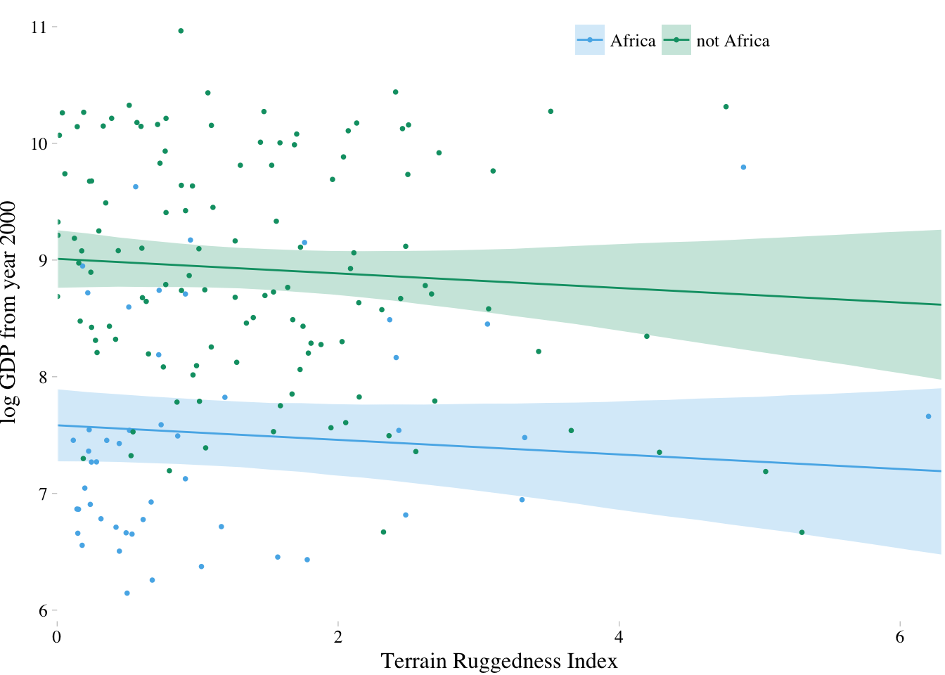
7.1.2. Adding a linear interaction does work
The model to fit here is:
\[\begin{eqnarray} { Y }_{ i } & \sim & Normal({ \mu }_{ i },\sigma ) & \text{<- likelihood } \\ { \mu }_{ i } & = & \alpha +\gamma_i { R }_{ i } +\beta_A { A }_{ i } & \text{<- linear model of } \mu \\ { \gamma }_{ i } & = & \beta_R +\beta_{AR} { A }_{ i } & \text{<- linear model of slope} \end{eqnarray}\]
The equation for \(\gamma_i\) defines the interaction between ruggedness and African nations. It is a linear interaction effect, because the equation \(\gamma_i\) is a linear model. By defining the relationship between GDP and ruggedness in this way, you are explicitly modeling the hypothesis that the slope between GDP and ruggedness depends (is conditional) upon whether or not a nation is in Africa.
For the priors, notice that I’m using weakly regularizing priors for the coefficients, and a very flat prior for the intercept.
We usually don’t know where the intercept will end up. But if we regularize on the coefficients, then the intercept will be effectively regularized by them.
m7.5 <-
    brm(data = dd, family = gaussian,
        log_gdp ~ 1 + rugged*cont_africa, # also works 1 + rugged + cont_africa + rugged:cont_africa
        prior = c(set_prior("normal(8, 100)", class = "Intercept"),
                  set_prior("normal(0, 1)", class = "b"),
                  set_prior("cauchy(0, 1)", class = "sigma")),
        chains = 4, iter = 2000, warmup = 1000, cores = 4)

plot(m7.5)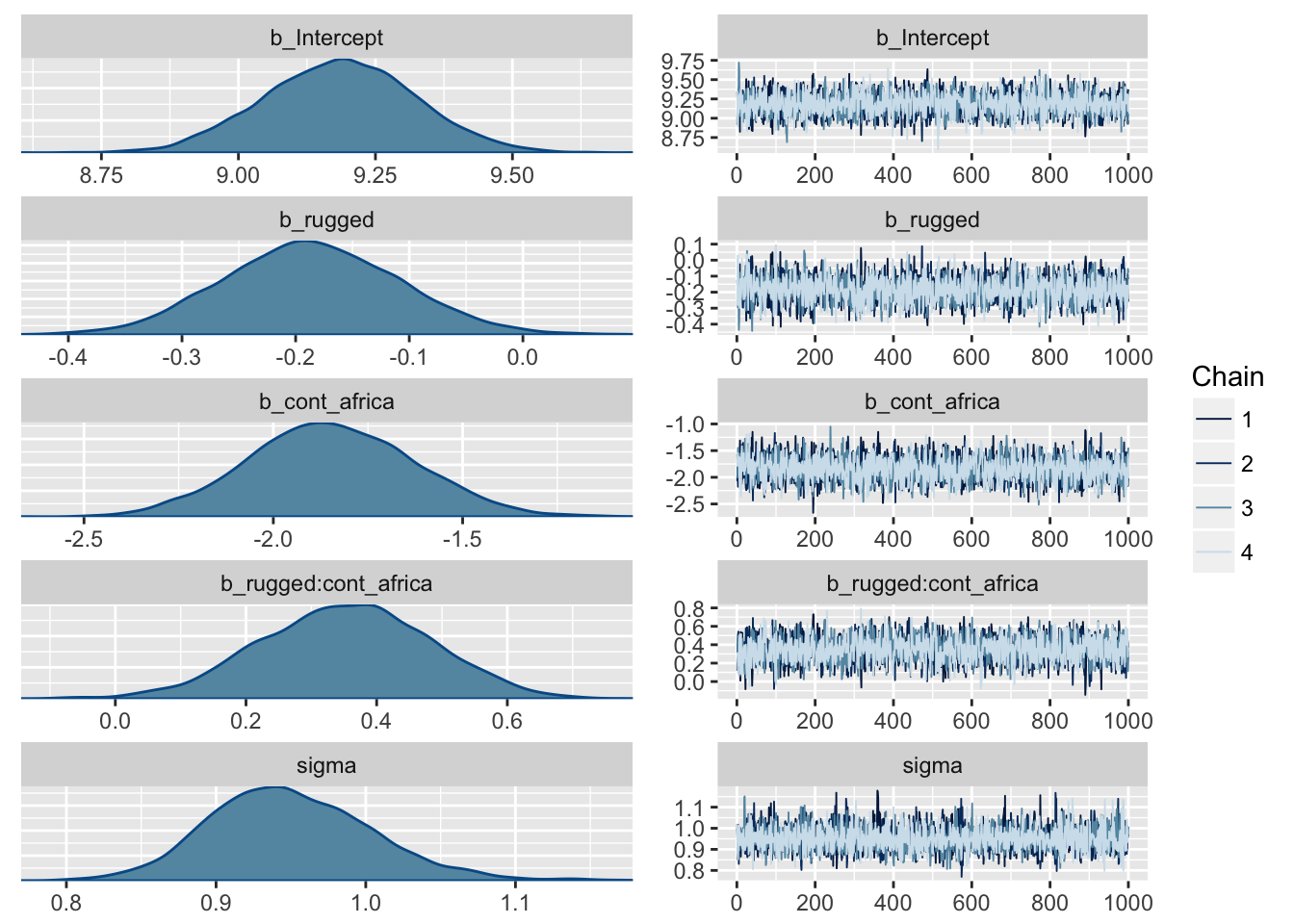
# ... are the fitted models
compare_waic <- function (..., sort = "WAIC", func = "WAIC")
{
    mnames <- as.list(substitute(list(...)))[-1L]

    L <- list(...)
    if (is.list(L[[1]]) && length(L) == 1) {L <- L[[1]]}

    classes <- as.character(sapply(L, class))
    if (any(classes != classes[1])) {
        warning("Not all model fits of same class.\nThis is usually a bad idea, because it implies they were fit by different algorithms.\nCheck yourself, before you wreck yourself.")
    }

    nobs_list <- try(sapply(L, nobs))
    if (any(nobs_list != nobs_list[1])) {
        nobs_out <- paste(mnames, nobs_list, "\n")
        nobs_out <- concat(nobs_out)
        warning(concat("Different numbers of observations found for at least two models.\nInformation criteria only valid for comparing models fit to exactly same observations.\nNumber of observations for each model:\n",
                       nobs_out))
    }

    dSE.matrix <- matrix(NA, nrow = length(L), ncol = length(L))

    if (func == "WAIC") {
        WAIC.list <- lapply(L, function(z) WAIC(z, pointwise = TRUE))
        p.list <- sapply(WAIC.list, function(x) x$p_waic)
        se.list <- sapply(WAIC.list, function(x) x$se_waic)
        IC.list <- sapply(WAIC.list, function(x) x$waic)
        #mnames <- sapply(WAIC.list, function(x) x$model_name)
        colnames(dSE.matrix) <- mnames
        rownames(dSE.matrix) <- mnames
        for (i in 1:(length(L) - 1)) {
            for (j in (i + 1):length(L)) {
                waic_ptw1 <- WAIC.list[[i]]$pointwise[ , 3]
                waic_ptw2 <- WAIC.list[[j]]$pointwise[ , 3]
                dSE.matrix[i, j] <- as.numeric(sqrt(length(waic_ptw1) *
                                                        var(waic_ptw1 - waic_ptw2)))
                dSE.matrix[j, i] <- dSE.matrix[i, j]
            }
        }
    }

    #if (!(the_func %in% c("DIC", "WAIC", "LOO"))) {
    #    IC.list <- lapply(L, function(z) func(z))
    #}
    IC.list <- unlist(IC.list)
    dIC <- IC.list - min(IC.list)
    w.IC <- rethinking::ICweights(IC.list)
    if (func == "WAIC") {
        topm <- which(dIC == 0)
        dSEcol <- dSE.matrix[, topm]
        result <- data.frame(WAIC = IC.list, pWAIC = p.list,
                             dWAIC = dIC, weight = w.IC, SE = se.list, dSE = dSEcol)
    }

    #if (!(the_func %in% c("DIC", "WAIC", "LOO"))) {
    #    result <- data.frame(IC = IC.list, dIC = dIC, weight = w.IC)
    #}
    rownames(result) <- mnames
    if (!is.null(sort)) {
        if (sort != FALSE) {
            if (sort == "WAIC")
                sort <- func
            result <- result[order(result[[sort]]), ]
        }
    }
    new("compareIC", output = result, dSE = dSE.matrix)
}

compare_waic(m7.3, m7.4, m7.5)
## Warning: Accessing p_waic using '$' is deprecated and will be removed in
## a future release. Please extract the p_waic estimate from the 'estimates'
## component instead.
## Warning: Accessing p_waic using '$' is deprecated and will be removed in
## a future release. Please extract the p_waic estimate from the 'estimates'
## component instead.
## Warning: Accessing p_waic using '$' is deprecated and will be removed in
## a future release. Please extract the p_waic estimate from the 'estimates'
## component instead.## Warning: Accessing se_waic using '$' is deprecated and will be removed in
## a future release. Please extract the se_waic estimate from the 'estimates'
## component instead.
## Warning: Accessing se_waic using '$' is deprecated and will be removed in
## a future release. Please extract the se_waic estimate from the 'estimates'
## component instead.
## Warning: Accessing se_waic using '$' is deprecated and will be removed in
## a future release. Please extract the se_waic estimate from the 'estimates'
## component instead.## Warning: Accessing waic using '$' is deprecated and will be removed in
## a future release. Please extract the waic estimate from the 'estimates'
## component instead.
## Warning: Accessing waic using '$' is deprecated and will be removed in
## a future release. Please extract the waic estimate from the 'estimates'
## component instead.
## Warning: Accessing waic using '$' is deprecated and will be removed in
## a future release. Please extract the waic estimate from the 'estimates'
## component instead.## WAIC pWAIC dWAIC weight SE dSE
## m7.5 469.2 5.0 0.0 0.97 14.60 NA
## m7.4 476.2 4.2 7.0 0.03 14.81 6.05
## m7.3 539.5 2.6 70.3 0.00 12.92 14.63The modicum of weight given to m7.4 suggests that the posterior means for the slopes in m7.5 are a little overfit. And the standard error of the difference in WAIC between the top two models is almost the same as the difference itself. There are only so many African countries, after all, so the data are sparse as far as estimating the interaction goes.
7.1.3 Plotting the interaction
Check also the Bonus section: Marginal Effects.
nd <-
    tibble(rugged = rep(seq(from = 0,
                            to = 6.3,
                            length.out = 30),
                        times = 2),
           cont_africa = rep(0:1, each = 30))

fit.7.5 <- fitted(m7.5, newdata = nd) %>%
    as_tibble() %>%
    bind_cols(nd) %>%
    mutate(cont_africa = ifelse(cont_africa == 1, "Africa", "not Africa"))

dd %>%
  mutate(cont_africa = ifelse(cont_africa == 1, "Africa", "not Africa")) %>%
  ggplot(aes(x = rugged)) +
  theme_pander() +
  scale_colour_pander() +
  scale_fill_pander() +
  geom_ribbon(data = fit.7.5,
              aes(ymin = `2.5%ile`,
                  ymax = `97.5%ile`,
                  fill = cont_africa,
                  group = cont_africa),
              alpha = 1/4) +
  geom_line(data = fit.7.5,
              aes(y = Estimate,
                  color = cont_africa,
                  group = cont_africa)) +
  geom_point(aes(y = log_gdp, color = cont_africa),
             size = 2/3) +
  scale_x_continuous(expand = c(0, 0)) +
  labs(x = "Terrain Ruggedness Index",
       y = "log GDP from year 2000") +
  theme(text = element_text(family = "Times"),
        legend.position = "none") +
  facet_wrap(~cont_africa)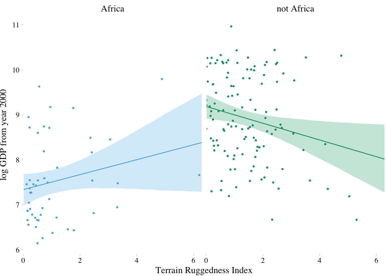
7.1.4. Interpreting an interaction estimate
Interpreting interaction estimates is tricky. There are two basic reasons to be wary of interpreting tables of posterior means and standard deviations as a way to understanding interactions.
- When you add an interaction to a model, this changes the meanings of the parameters. A “main effect” coefficient in an interaction model does not mean the same thing as a coefficient of the same name in a model without an interaction. Their distributions cannot usually be directly compared.
- Tables of numbers don’t make it easy to fully incorporate uncertainty in our thinking, since covariance among parameters isn’t usually shown. And this gets much harder once the influence of a predictor depends upon multiple parameters.
7.1.4.1. Parameters change meaning
p7.5 <- posterior_samples(m7.5)

p7.5 %>%
    mutate(gamma_Africa = b_rugged + `b_rugged:cont_africa`,
           gamma_notAfrica = b_rugged) %>%
    select(gamma_Africa, gamma_notAfrica) %>%
    gather(key, value) %>%
    group_by(key) %>%
    summarise(mean = mean(value))
## # A tibble: 2 x 2
## key mean
## <chr> <dbl>
## 1 gamma_Africa 0.166
## 2 gamma_notAfrica -0.1867.1.4.2. Incorporating uncertainty
p7.5 %>%
    mutate(gamma_Africa = b_rugged + `b_rugged:cont_africa`,
           gamma_notAfrica = b_rugged) %>%
    select(gamma_Africa, gamma_notAfrica) %>%
    gather(key, value) %>%
    ggplot(aes(x = value, group = key, color = key, fill = key)) +
    theme_pander() +
    scale_color_pander() +
    scale_fill_pander() +
    geom_density(alpha = 1/4) +
    scale_x_continuous(expression(gamma), expand = c(0, 0)) +
    scale_y_continuous(NULL, breaks = NULL) +
    labs(title = "Terraine Ruggedness slopes",
         subtitle = "Blue = African nations, Green = others") +
    theme(text = element_text(family = "Times"))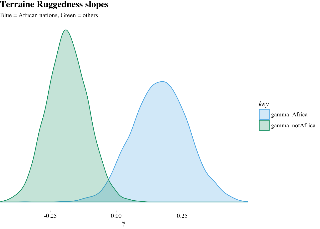
The distributions in the figure are marginal, like silhouettes of each distribution, ignoring all of the other dimensions in the posterior.
What proportion of these differences is below zero?
p7.5 %>%
    mutate(gamma_Africa = b_rugged + `b_rugged:cont_africa`,
           gamma_notAfrica = b_rugged,
           diff = gamma_Africa - gamma_notAfrica) %>%
    summarise(Proportion_of_the_difference_below_0 = sum(diff < 0)/length(diff))
## Proportion_of_the_difference_below_0
## 1 0.00375So conditional on this model and these data, it’s highly implausible that the slope association ruggedness with log-GDP is lower inside Africa than outside it. In other words, what the golem is telling is that it is very skeptical of the notion that \(\gamma\) within Africa is lower than \(\gamma\) outside of Africa. How skeptical? Of all the possible states of the world it knows about, only a 0.36% of them are consistent with both the data and the claim that \(\gamma\) in Africa is less than \(\gamma\) outside Africa. Your golem is skeptical, but it’s usually a good idea for you to remain skeptical of your golem.
7.2. Symmetry of the linear interaction
For the model above, the interaction has two equally valid phrasings:
- How much does the influence of ruggedness (on GDP) depend upon whether the nation is in Africa?
- How much does the influence of being in Africa (on GDP) depend upon ruggedness?
nd <-
    tibble(rugged = rep(range(dd$rugged), times = 2),
           cont_africa = rep(c(0,1), each = 2),
           ruggedness = rep(c("Minimum", "Maximum"), times = 2))

fit.7.5 <- fitted(m7.5, newdata = nd) %>%
    as_tibble() %>%
    bind_cols(nd) %>%
    mutate(cont_africa = ifelse(cont_africa == 1, "Africa", "not Africa"))

dd %>%
    mutate(cont_africa = ifelse(cont_africa == 1, "Africa", "not Africa")) %>%
    ggplot(aes(x = cont_africa)) +
    theme_pander() +
    scale_colour_pander() +
    scale_fill_pander() +
    geom_point(aes(y = log_gdp),
             size = 2/3) +
    geom_ribbon(data = fit.7.5,
              aes(ymin = `2.5%ile`,
                  ymax = `97.5%ile`,
                  fill = ruggedness,
                  group = ruggedness),
              alpha = 1/4) +
    geom_line(data = fit.7.5,
              aes(y = Estimate,
                  color = ruggedness,
                  group = ruggedness)) +
    labs(x = "Continent",
       y = "log GDP from year 2000") +
    theme(text = element_text(family = "Times"))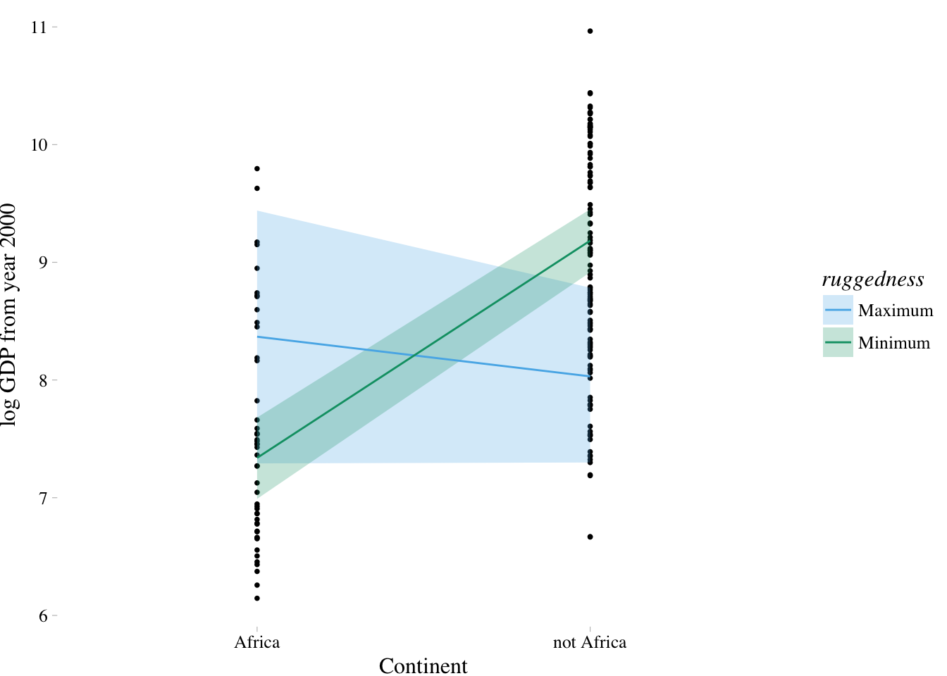
7.3. Continuous interactions
Benefits of centering prediction variables:
- First, centering the prediction variables can make it much easier to lean on the coefficients alone in understanding the model, especially when you want to compare the estimates from models with and without an interaction.
- Second, sometimes model fitting has a hard time with uncentered variables. Centering (and possibly also standardizing) the data before fitting the model can help you achieve a faster and more reliable set of estimates.
7.3.1. The data
library(rethinking)
data(tulips)
d <- tulips
detach(package:rethinking, unload = T)
rm(tulips)
glimpse(d)
## Observations: 27
## Variables: 4
## $ bed <fct> a, a, a, a, a, a, a, a, a, b, b, b, b, b, b, b, b, b, c...
## $ water <int> 1, 1, 1, 2, 2, 2, 3, 3, 3, 1, 1, 1, 2, 2, 2, 3, 3, 3, 1...
## $ shade <int> 1, 2, 3, 1, 2, 3, 1, 2, 3, 1, 2, 3, 1, 2, 3, 1, 2, 3, 1...
## $ blooms <dbl> 0.00, 0.00, 111.04, 183.47, 59.16, 76.75, 224.97, 83.77...7.3.2. The un-centered models
Priors that look very flat may not actually be, because “flat” is always relative to the likelihood.
m7.6 <-
  brm(data = d, family = gaussian,
      blooms ~ 1 + water + shade,
      prior = c(set_prior("normal(0, 100)", class = "Intercept"),
                set_prior("normal(0, 100)", class = "b"),
                set_prior("cauchy(0, 10)", class = "sigma")),
      iter = 2000, warmup = 1000, cores = 4, chains = 4,
      control = list(adapt_delta = 0.9))

m7.7 <-
  brm(data = d, family = gaussian,
      blooms ~ 1 + water + shade + water:shade,
      prior = c(set_prior("normal(0, 100)", class = "Intercept"),
                set_prior("normal(0, 100)", class = "b"),
                set_prior("cauchy(0, 10)", class = "sigma")),
      iter = 2000, warmup = 1000, cores = 4, chains = 4,
      control = list(adapt_delta = 0.9))
fixef(m7.6) %>% round(digits = 2)## Estimate Est.Error 2.5%ile 97.5%ile
## Intercept 60.84 42.18 -22.16 143.02
## water 73.84 14.28 45.08 101.82
## shade -40.65 14.77 -69.40 -11.42fixef(m7.7) %>% round(digits = 2)## Estimate Est.Error 2.5%ile 97.5%ile
## Intercept -108.49 60.99 -222.70 15.56
## water 160.72 28.47 103.32 214.32
## shade 44.72 28.28 -12.77 98.16
## water:shade -43.62 13.20 -67.61 -15.837.3.3. Center and re-estimate
d <-
  d %>%
  mutate(shade.c = shade - mean(shade),
         water.c = water - mean(water))

m7.8 <-
  brm(data = d, family = gaussian,
      blooms ~ 1 + water.c + shade.c,
      prior = c(set_prior("normal(130, 100)", class = "Intercept"),
                set_prior("normal(0, 100)", class = "b"),
                set_prior("cauchy(0, 10)", class = "sigma")),
      chains = 4, iter = 2000, warmup = 1000, cores = 4,
      control = list(adapt_delta = 0.9))

m7.9 <-
  brm(data = d, family = gaussian,
      blooms ~ 1 + water.c + shade.c + water.c:shade.c,
      prior = c(set_prior("normal(130, 100)", class = "Intercept"),
                set_prior("normal(0, 100)", class = "b"),
                set_prior("cauchy(0, 10)", class = "sigma")),
      chains = 4, iter = 2000, warmup = 1000, cores = 4,
      control = list(adapt_delta = 0.9))
fixef(m7.8) %>% round(digits = 2)## Estimate Est.Error 2.5%ile 97.5%ile
## Intercept 128.77 11.89 105.55 152.07
## water.c 74.07 14.41 45.23 102.86
## shade.c -40.86 14.49 -69.29 -12.09fixef(m7.9) %>% round(digits = 2)## Estimate Est.Error 2.5%ile 97.5%ile
## Intercept 129.02 9.82 109.80 148.10
## water.c 74.62 11.86 50.25 97.61
## shade.c -41.39 12.04 -64.40 -17.67
## water.c:shade.c -52.02 14.67 -80.95 -23.31The explanation of the coefficients is as follows:
- The Intercept is the expected value of blooms when both water and shade are at their average values. Their average values are both zero (0), because they were centered before fitting the model.
- The estimate
water.cis the expected change in blooms when water increases by one unit and shade is at its average value (of zero). This parameter does not tell you the expected rate of change for any other value of shade. This estimate suggests that when shade is at its average value, increasing water is highly beneficial to blooms.- The estimate
shade.cis the expected change in blooms when shade increases by one unit and water is at its average value (of zero). This parameter does not tell you the expected rate of change for any other value of water. This estimate suggests that when water is at its average value, increasing shade is highly detrimental to blooms.- The estimate
water.c:shade.cis the interaction effect. Like all linear interactions, it can be explained in more than one way. First, the estimate tells us the expected change in the influence of water on blooms when increasing shade by one unit. Second, it tells us the expected change in the influence of shade on blooms when increasing water by one unit. So why is the interaction estimate,water.c:shade.c, negative? The short answer is that water and shade have opposite effects on blooms, but that each also makes the other more important to the outcome.
7.3.4. Plotting implied predictions
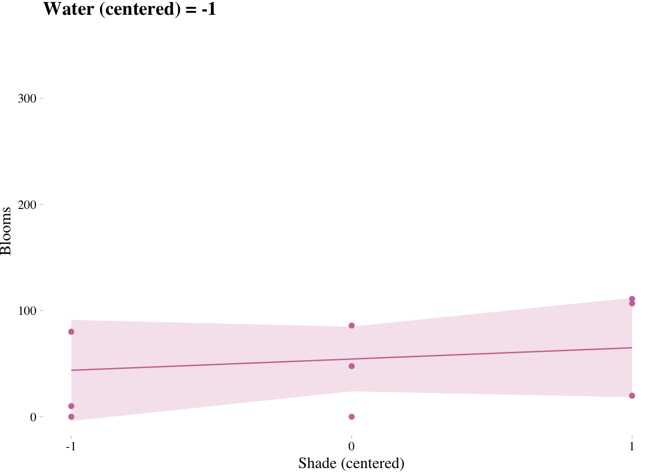
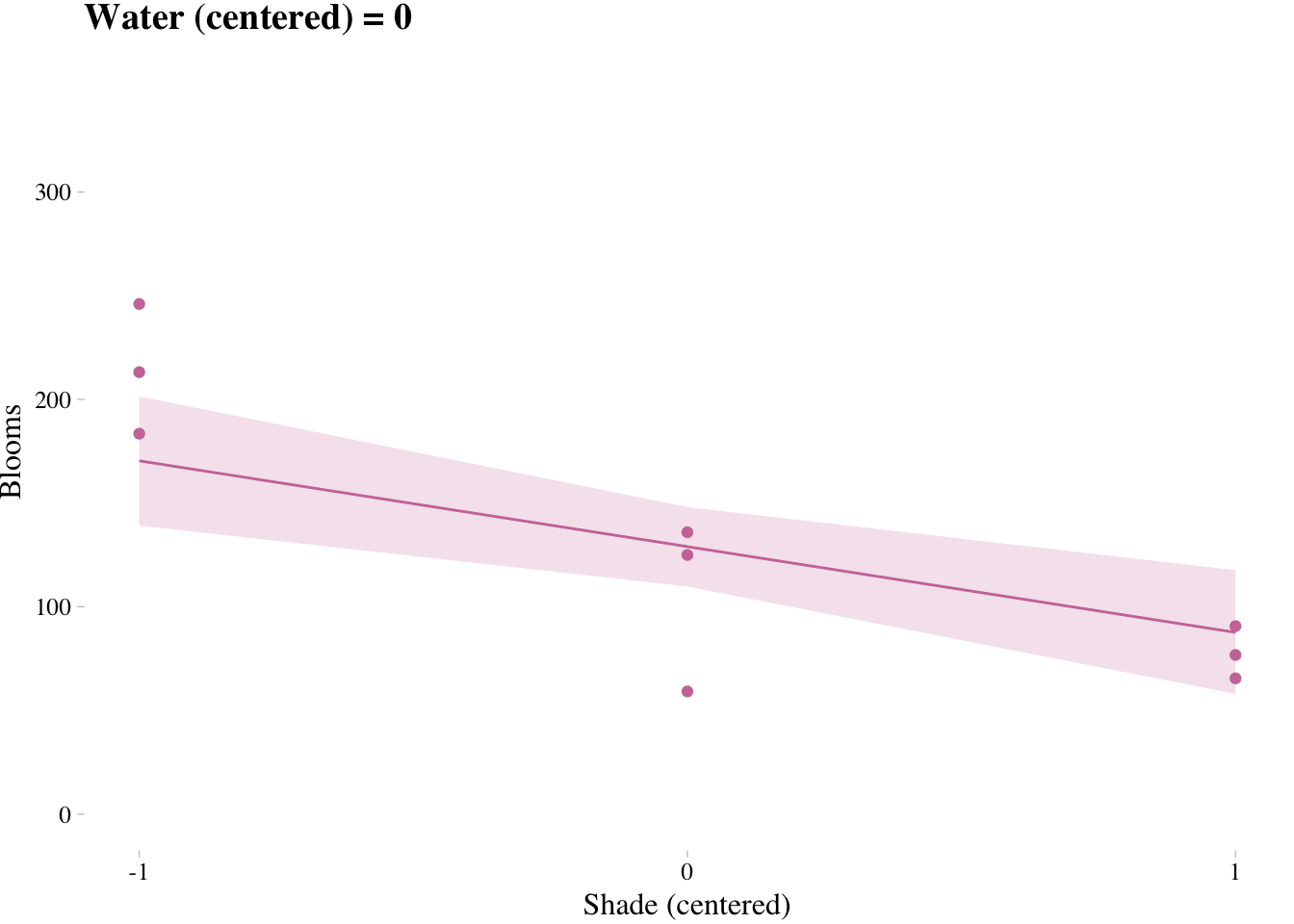
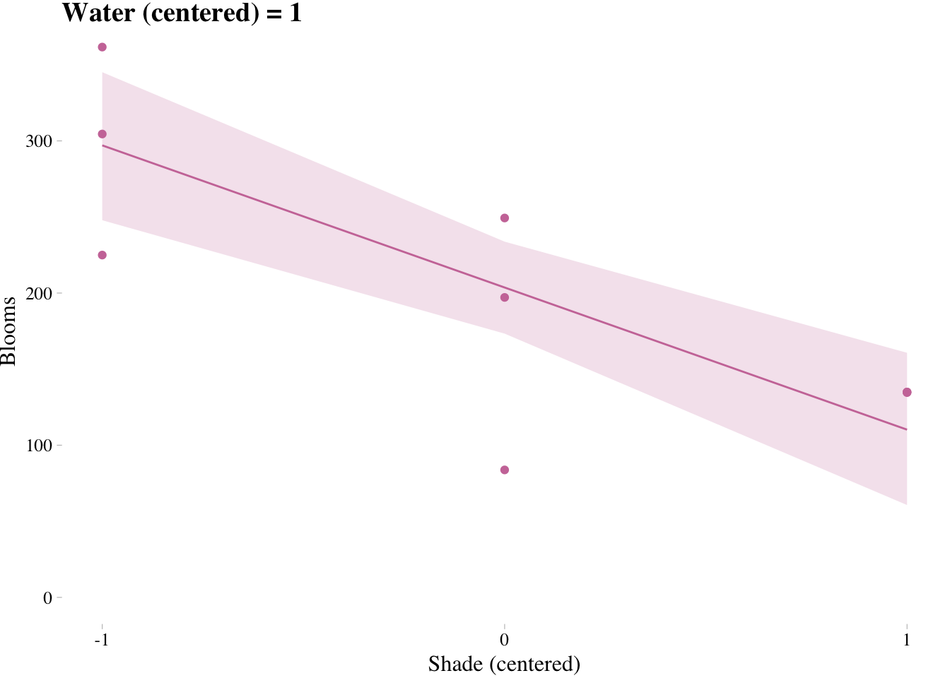
Triptych plots are very handy for understanding the impact of interactions.
# loop over values of waterC and plot predictions
shade.seq <- -1:1

for(w in -1:1){
  # defining the subset of the original data
  dt <- d[d$water.c == w, ]
  # defining our new data
  nd <- tibble(water.c = w, shade.c = shade.seq)
  # using our sampling skills, like before
  fit.7.9 <- fitted(m7.9, newdata = nd) %>%
    as_tibble() %>%
    bind_cols(nd)

  # specifying our custom plot
  fig <- ggplot() + # can't seem to get the name to work dynamically (e.g., paste("fig", w, sep = "_") returns an error). Hit a brother up if you can figure out how to code this correctly such that the loop returns three objects: fig_-1, fig_0, and fig_1
    theme_pander() +
    geom_ribbon(data = fit.7.9,
                aes(x = shade.c,
                    ymin = `2.5%ile`,
                    ymax = `97.5%ile`),
                fill = "#CC79A7", alpha = 1/5) +
    geom_line(data = fit.7.9, aes(x = shade.c, y = Estimate),
              color = "#CC79A7") +
    geom_point(data = dt, aes(x = shade.c, y = blooms),
               color = "#CC79A7") +
    coord_cartesian(xlim = c(-1, 1), ylim = c(0, 350)) +
    scale_x_continuous(breaks = c(-1, 0, 1)) +
    labs(x = "Shade (centered)", y = "Blooms",
         title = paste("Water (centered) =", w)) +
    theme(text = element_text(family = "Times"))

  # plotting that joint
  plot(fig)
}
Interaction terms can be visualized using the following code:
x <- z <- w <- 1
colnames( model.matrix(~x*z*w) )
Bonus: Marginal Effects
The brms package includes the marginal_effects() function as a convenient way to look at simple effects and two-way interactions.
marginal_effects(m7.3)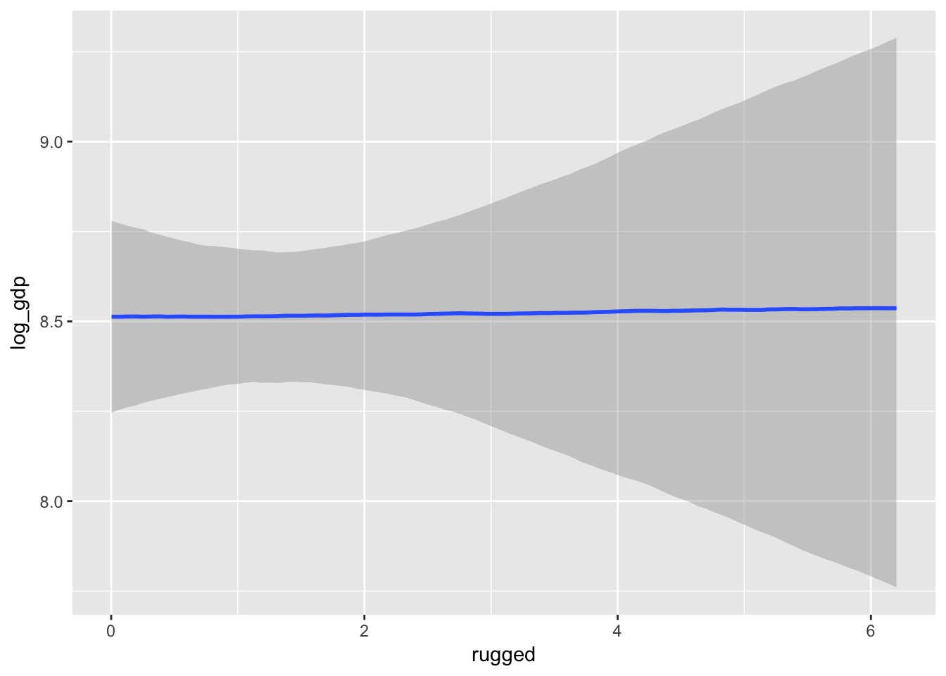
plot(marginal_effects(m7.3, spaghetti = T, nsamples = 200),
     points = T,
     point_args = c(alpha = 1/2, size = 1))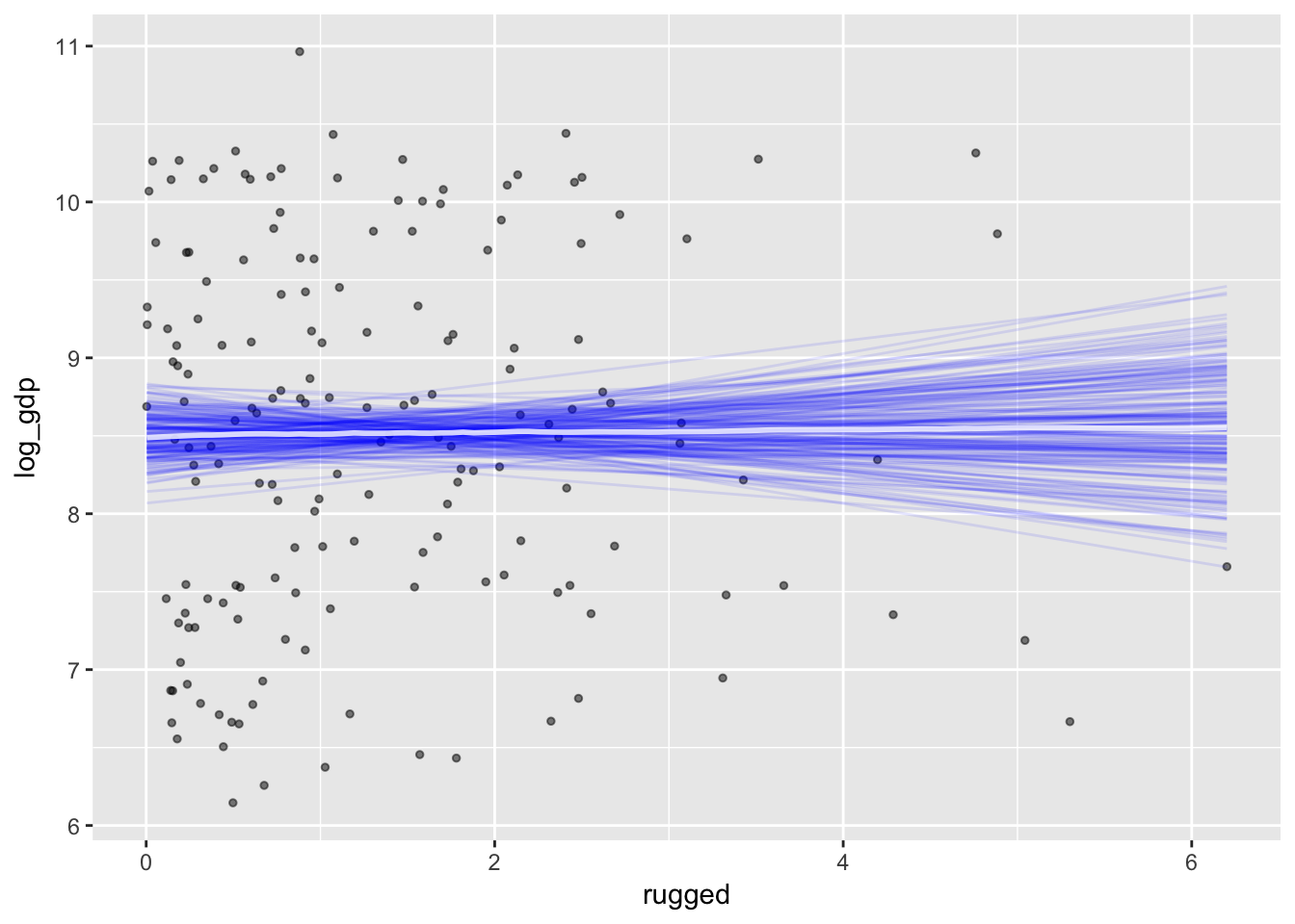
d_factor <-
  m7.4$data %>%
  mutate(cont_africa = factor(cont_africa))

m7.4_factor <-
  brm(data = d_factor, family = gaussian,
      log_gdp ~ 1 + rugged + cont_africa,
      prior = c(set_prior("normal(8, 100)", class = "Intercept"),
                set_prior("normal(0, 1)", class = "b"),
                set_prior("cauchy(0, 10)", class = "sigma")),
      chains = 4, iter = 2000, warmup = 1000, cores = 4)

d_factor <-
  m7.5$data %>%
  mutate(cont_africa = factor(cont_africa))

m7.5_factor <-
  brm(data = d_factor, family = gaussian,
      log_gdp ~ 1 + rugged*cont_africa,
      prior = c(set_prior("normal(8, 100)", class = "Intercept"),
                set_prior("normal(0, 1)", class = "b"),
                set_prior("cauchy(0, 10)", class = "sigma")),
      chains = 4, iter = 2000, warmup = 1000, cores = 4)
# plot(marginal_effects(m7.4_factor))
# marginal_effects(m7.5_factor, probs = c(.25, .75))
plot(marginal_effects(m7.5_factor,
effects = "rugged:cont_africa",
spaghetti = T, nsamples = 150),
points = T,
point_args = c(alpha = 2/3, size = 1), mean = F)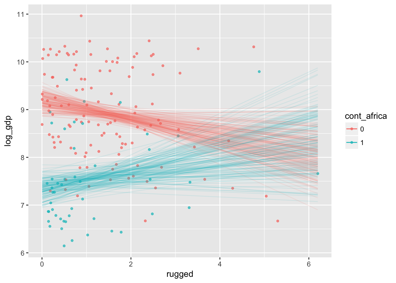
ic <- list(water.c = c(-1, 0, 1))
plot(marginal_effects(m7.9,
                      effects = "shade.c:water.c",
                      int_conditions = ic),
     points = T)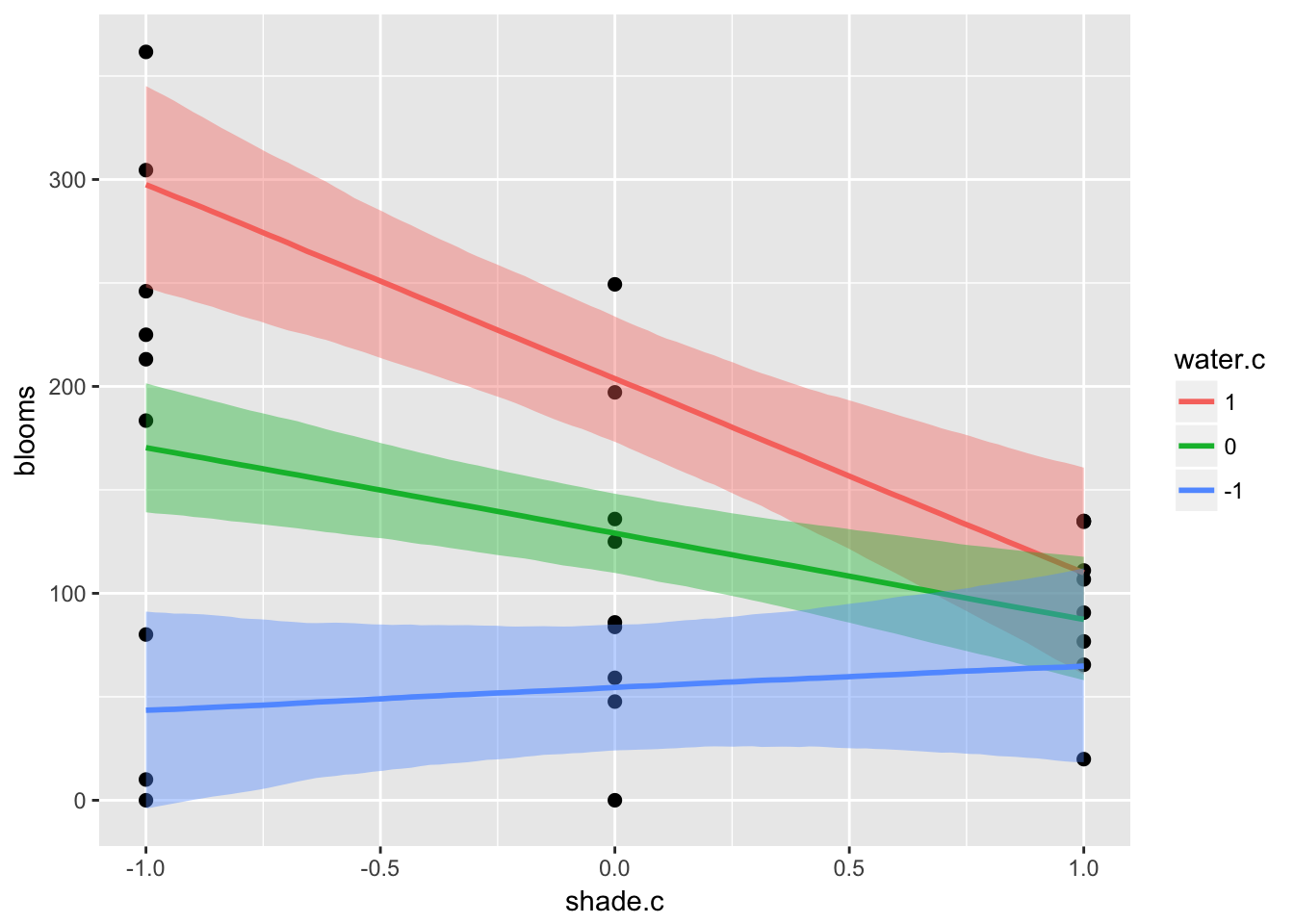
ic <- list(shade.c = c(-1, 0, 1))
plot(marginal_effects(m7.9,
                      effects = "water.c:shade.c",
                      int_conditions = ic),
     points = T)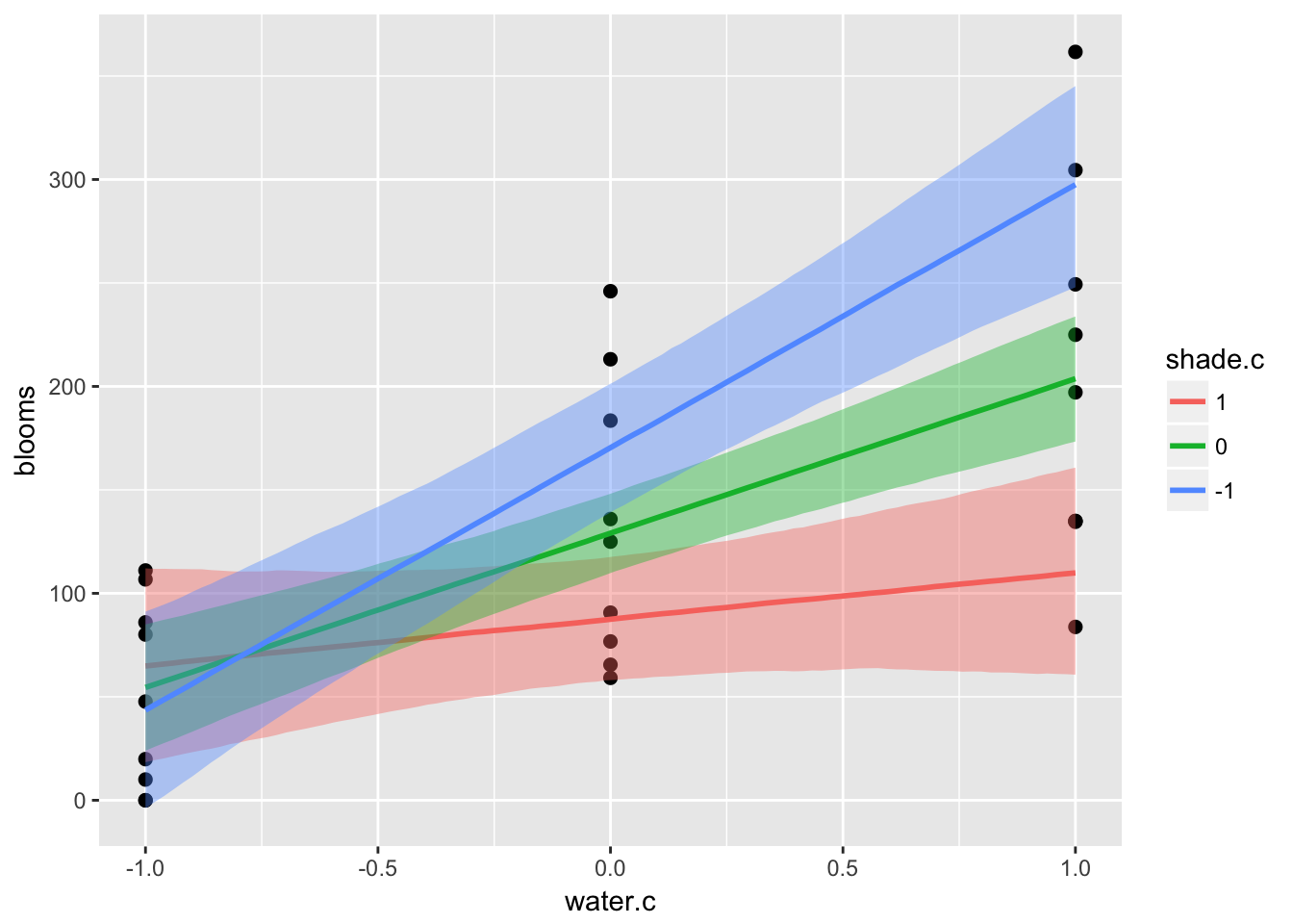
References
McElreath, R. (2016). Statistical rethinking: A Bayesian course with examples in R and Stan. Chapman & Hall/CRC Press.
Kurz, A. S. (2018, March 9). brms, ggplot2 and tidyverse code, by chapter. Retrieved from https://goo.gl/JbvNTj