Notes on Statistical Rethinking (Chapter 8 - Markov Chain Monte Carlo)

Apr 19, 2018 33 min read StatisticalRethinking

The Stan programming language is not an abbreviation or acronym. Rather, it is named after Stanislaw Ulam (1909–1984). Ulam is credited as one of the inventors of Markov chain Monte Carlo. Together with Ed Teller, Ulam applied it to designing fusion bombs. But he and others soon applied the general Monte Carlo method to diverse problems of less monstrous nature. Ulam made important contributions in pure mathematics, chaos theory, and molecular and theoretical biology, as well.

The Markov-chain Monte Carlo Interactive Gallery.

8.1. Good King Markov and His island kingdom

The Metropolis algorithm:

Wherever the King is, each week he decides between staying put for another week or moving to one of the two adjacent islands. To decide his next move, he flips a coin.

If the coin turns up heads, the King considers moving to the adjacent island clockwise around the archipelago. If the coin turns up tails, he considers instead moving counterclockwise. Call the island the coin nominates the proposal island.

Now, to see whether or not he moves to the proposal island, King Markov counts out a number of seashells equal to the relative population size of the proposal island. So for example, if the proposal island is number 9, then he counts out 9 seashells. Then he also counts out a number of stones equal to the relative population of the current island. So for example, if the current island is number 10, then King Markov ends up holding 10 stones, in addition to the 9 seashells.

When there are more seashells than stones, King Markov always moves to the proposal island. But if there are fewer shells than stones, he discards a number of stones equal to the number of shells. So for example, if there are 4 shells and 6 stones, he ends up with 4 shells and 6 - 4 = 2 stones. Then he places the shells and the remaining stones in a bag. He reaches in and randomly pulls out one object. If it is a shell, he moves to the proposal island. Otherwise, he stays put another week. As a result, the probability that he moves is equal to the number of shells divided by the original number of stones.

set.seed(103)

num_weeks <- 1e5
positions <- rep(0, num_weeks)
current   <- 10
for (i in 1:num_weeks) {
    # record current position
    positions[i] <- current
  
    # flip coin to generate proposal
    proposal <- current + sample(c(-1, 1), size = 1)
  
    # now make sure he loops around the archipelago
    if (proposal < 1) proposal <- 10
    if (proposal > 10) proposal <- 1
  
    # move?
    prob_move <- proposal/current
    current <- ifelse(runif(1) < prob_move, proposal, current)
}

library(hrbrthemes)
library(tidyverse)

tibble(week = 1:1e5,
       island = positions) %>%
    filter(week < 101) %>%
    ggplot(aes(x = week, y = island)) +
    geom_point(shape = 1) +
    geom_line() +
    scale_x_continuous(breaks = seq(from = 0, to = 100, by = 20)) +
    scale_y_continuous(breaks = seq(from = 0, to = 10, by = 2)) +
    labs(title = "Behold: The Metropolis algorithm in action!",
         subtitle = "The dots show the king's path over the first 100 weeks.") +
    theme_ipsum()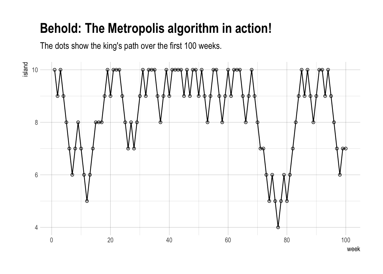

tibble(week = 1:1e5,
       island = positions) %>%
    mutate(island = factor(island)) %>%
    ggplot(aes(x = island)) +
    geom_bar() +
    labs(title = "Old Metropolis shines in the long run.",
         subtitle = "Sure enough, the time the king spent on each island was\nproportional to its population size.") +
    theme_ipsum()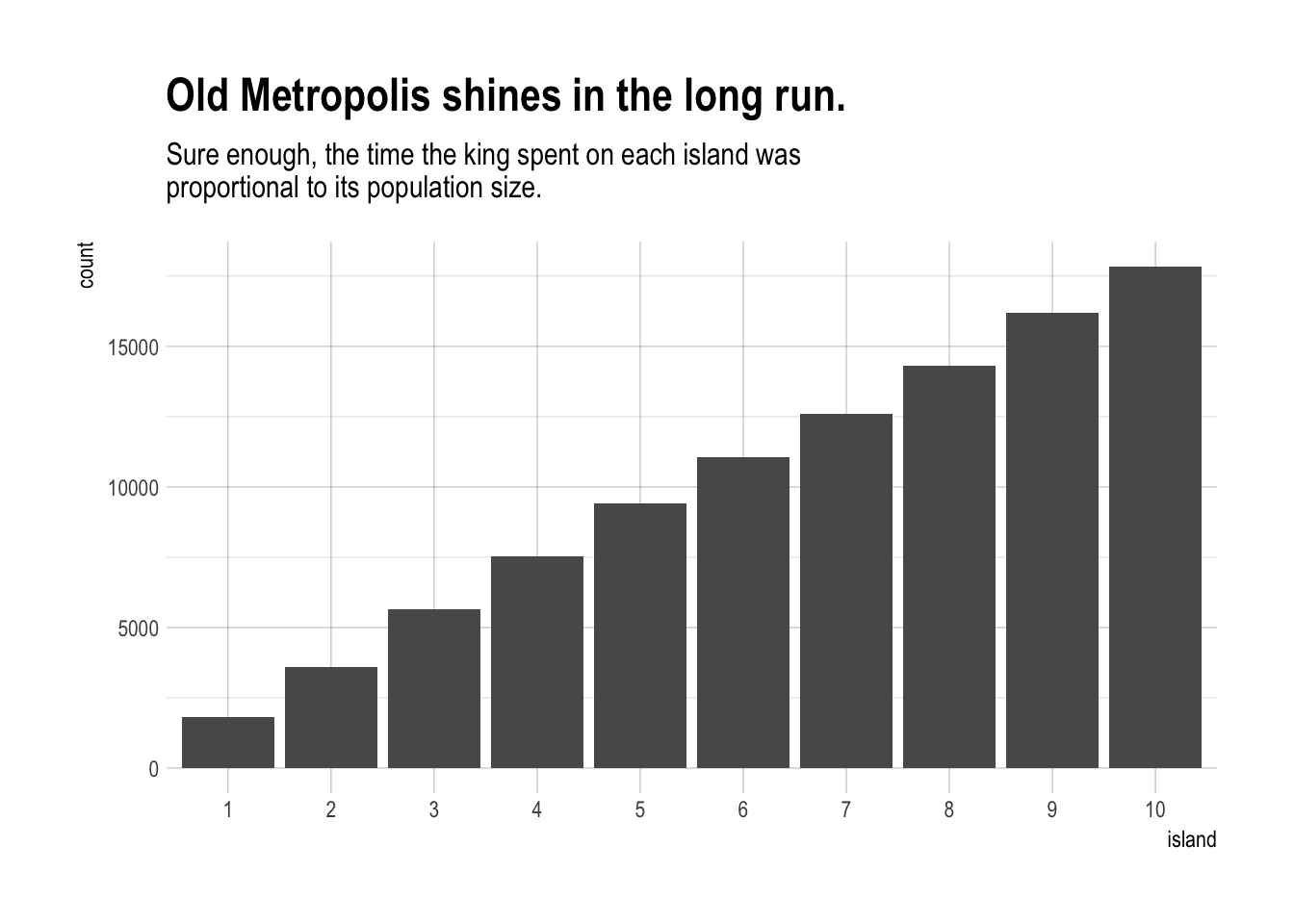

8.2. Markov chain Monte Carlo

The precise algorithm King Markov used is a special case of the general Metropolis algorithm from the real world. And this algorithm is an example of Markov chain Monte Carlo. In real applications, the goal is to draw samples from an unknown and usually complex target distribution, like a posterior probability distribution.

The “islands” in our objective are parameter values, and they need not be discrete, but can instead take on a continuous range of values as usual.

The “population sizes” in our objective are the posterior probabilities at each parameter value.

The “weeks” in our objective are samples taken from the joint posterior of the parameters in the model.

Provided the way we choose our proposed parameter values at each step is symmetric, so that there is an equal chance of proposing from A to B and from B to A, then the Metropolis algorithm will eventually give us a collection of samples from the joint posterior.

8.2.1. Gibbs sampling

The Metropolis algorithm works whenever the probability of proposing a jump to B from A is equal to the probability of proposing A from B, when the proposal distribution is symmetric. There is a more general method, known as Metropolis-Hastings, that allows asymmetric proposals. This would mean, in the context of King Markov’s fable, that the King’s coin were biased to lead him clockwise on average. One reason such a choice is that it makes it easier to handle parameters, like standard deviations, that have boundaries at zero. A better reason, however, is that it allows us to generate savvy proposals that explore the posterior distribution more efficiently. By “more efficiently,” I mean that we can acquire an equally good image of the posterior distribution in fewer steps.

Gibbs sampling is a variant of the Metropolis-Hastings algorithm that uses clever proposals and is therefore more efficient. By “efficient,” I mean that you can get a good estimate of the posterior from Gibbs sampling with many fewer samples than a comparable Metropolis approach. The improvement arises from adaptive proposals in which the distribution of proposed parameter values adjusts itself intelligently, depending upon the parameter values at the moment. How Gibbs sampling computes these adaptive proposals depends upon using particular combinations of prior distributions and likelihoods known as conjugate pairs.

But there are some severe limitations to Gibbs sampling. First, maybe you don’t want to use conjugate priors. Some conjugate priors seem silly, and choosing a prior so that the model fits efficiently isn’t really a strong argument from a scientific perspective. Second, as models become more complex and contain hundreds or thousands or tens of thousands of parameters, Gibbs sampling becomes shockingly inefficient.

8.2.2. Hamiltonian Monte Carlo

Check this blog post by R. McElreath.

Hamiltonian Monte Carlo (or Hybrid Monte Carlo, HMC) is much more computationally costly than are Metropolis or Gibbs sampling. But its proposals are typically much more efficient. As a result, it doesn’t need as many samples to describe the posterior distribution.

Consider a different fable. Suppose King Markov’s cousin Monty is King on the mainland. Monty’s kingdom is not a discrete set of islands. Instead, it is a continuous territory stretched out along a narrow valley. But the King has a similar obligation: to visit his citizens in proportion to their local density.

Also like Markov, Monty has a highly educated and mathematically gifted advisor. His name is Hamilton. Hamilton realized that a much more efficient way to visit the citizens in the continuous Kingdom is to travel back and forth along its length. In order to spend more time in densely settled areas, they should slow the royal vehicle down when houses grow more dense. Likewise, they should speed up when houses grow more sparse. This strategy requires knowing how quickly population density is changing, at their current location. But it doesn’t require remembering where they’ve been or knowing the population distribution anyplace else. And a major benefit of this strategy compared to that of Metropolis is that the King makes a full sweep of the kingdom before revisiting anyone.

In statistical applications, the royal vehicle is the current vector of parameter values. In the single parameter case, the log-posterior is like a bowl, with the MAP at its nadir (lowest point). Then the job is to sweep across the surface of the bowl, adjusting speed in proportion to how high up we are. HMC really does run a physics simulation, pretending the vector of parameters gives the position of a little frictionless particle. The log-posterior provides a surface for this particle to glide across. When the log-posterior is very flat, because there isn’t much information in the likelihood and the priors are rather flat, then the particle can glide for a long time before the slope (gradient) makes it turn around. When instead the log-posterior is very steep, because either the likelihood or the priors are very concentrated, then the particle doesn’t get far before turning around.

HMC requires continuous parameters. It can’t glide through a discrete parameter. In practice, this means that certain advanced techniques, like the imputation of discrete missing data, are not possible with HMC alone. And there are types of models that remain difficult for any MCMC strategy.

Check this blog post about how to sample discrete parameters with Hamiltonian Monte Carlo.

A big limitation of HMC is that it needs to be tuned to a particular model and its data. The frictionless particle does need mass, so it can acquire momentum, and the choice of mass can have big effects on efficiency. There are also a number of other parameters that define the HMC algorithm, but no the statistical model, that can change how efficiently the Markov chain samples. Tuning all of those parameters by hand is a pain. That’s where an engine like Stan (mc-stan.org) comes in.

8.3. Easy HMC: `brm()`

library(rethinking)
data(rugged)
d <- rugged

detach(package:rethinking)
library(brms)

## Warning: package 'Rcpp' was built under R version 3.4.4

rm(rugged)

d <- 
  d %>%
  mutate(log_gdp = log(rgdppc_2000))

dd <-
  d %>%
  filter(complete.cases(rgdppc_2000))

8.3.1. Preparation

There are some steps that need to be taken before fitting a model:

Preprocess all variable transformations. If the outcome is transformed somehow, like by taking the logarithm, then do this before fitting the model by constructing a new variable in the data frame. Likewise, if any predictor variables are transformed, including squaring and cubing and such to build polynomial models, then compute these transformed values before fitting the model.

Once you’ve got all the variables ready, make a new trimmed down data frame that contains only the variables you will actually use to fit the model. Technically, you don’t have to do this. But doing so avoids common problems. For example, if any of the unused variables have missing values, NA, then Stan will refuse to work.

dd.trim <-
  dd %>%
  select(log_gdp, rugged, cont_africa)

glimpse(dd.trim)

## Observations: 170
## Variables: 3
## $ log_gdp     <dbl> 7.492609, 8.216929, 9.933263, 9.407032, 7.792343, ...
## $ rugged      <dbl> 0.858, 3.427, 0.769, 0.775, 2.688, 0.006, 0.143, 3...
## $ cont_africa <int> 1, 0, 0, 0, 0, 0, 0, 0, 0, 1, 0, 1, 1, 0, 0, 0, 0,...

8.3.2. Estimation

m8.1 <- brm(data = dd.trim, 
            log_gdp ~ 1 + rugged + cont_africa + rugged:cont_africa,
            prior = c(set_prior("normal(0,100)", class = "Intercept"),
                      set_prior("normal(0,10)", class = "b"),
                      set_prior("cauchy(0,2)", class = "sigma")))

## 
## SAMPLING FOR MODEL 'gaussian brms-model' NOW (CHAIN 1).
## 
## Gradient evaluation took 4.8e-05 seconds
## 1000 transitions using 10 leapfrog steps per transition would take 0.48 seconds.
## Adjust your expectations accordingly!
## 
## 
## Iteration:    1 / 2000 [  0%]  (Warmup)
## Iteration:  200 / 2000 [ 10%]  (Warmup)
## Iteration:  400 / 2000 [ 20%]  (Warmup)
## Iteration:  600 / 2000 [ 30%]  (Warmup)
## Iteration:  800 / 2000 [ 40%]  (Warmup)
## Iteration: 1000 / 2000 [ 50%]  (Warmup)
## Iteration: 1001 / 2000 [ 50%]  (Sampling)
## Iteration: 1200 / 2000 [ 60%]  (Sampling)
## Iteration: 1400 / 2000 [ 70%]  (Sampling)
## Iteration: 1600 / 2000 [ 80%]  (Sampling)
## Iteration: 1800 / 2000 [ 90%]  (Sampling)
## Iteration: 2000 / 2000 [100%]  (Sampling)
## 
##  Elapsed Time: 0.096422 seconds (Warm-up)
##                0.091202 seconds (Sampling)
##                0.187624 seconds (Total)
## 
## 
## SAMPLING FOR MODEL 'gaussian brms-model' NOW (CHAIN 2).
## 
## Gradient evaluation took 1.5e-05 seconds
## 1000 transitions using 10 leapfrog steps per transition would take 0.15 seconds.
## Adjust your expectations accordingly!
## 
## 
## Iteration:    1 / 2000 [  0%]  (Warmup)
## Iteration:  200 / 2000 [ 10%]  (Warmup)
## Iteration:  400 / 2000 [ 20%]  (Warmup)
## Iteration:  600 / 2000 [ 30%]  (Warmup)
## Iteration:  800 / 2000 [ 40%]  (Warmup)
## Iteration: 1000 / 2000 [ 50%]  (Warmup)
## Iteration: 1001 / 2000 [ 50%]  (Sampling)
## Iteration: 1200 / 2000 [ 60%]  (Sampling)
## Iteration: 1400 / 2000 [ 70%]  (Sampling)
## Iteration: 1600 / 2000 [ 80%]  (Sampling)
## Iteration: 1800 / 2000 [ 90%]  (Sampling)
## Iteration: 2000 / 2000 [100%]  (Sampling)
## 
##  Elapsed Time: 0.103286 seconds (Warm-up)
##                0.092334 seconds (Sampling)
##                0.19562 seconds (Total)
## 
## 
## SAMPLING FOR MODEL 'gaussian brms-model' NOW (CHAIN 3).
## 
## Gradient evaluation took 1.6e-05 seconds
## 1000 transitions using 10 leapfrog steps per transition would take 0.16 seconds.
## Adjust your expectations accordingly!
## 
## 
## Iteration:    1 / 2000 [  0%]  (Warmup)
## Iteration:  200 / 2000 [ 10%]  (Warmup)
## Iteration:  400 / 2000 [ 20%]  (Warmup)
## Iteration:  600 / 2000 [ 30%]  (Warmup)
## Iteration:  800 / 2000 [ 40%]  (Warmup)
## Iteration: 1000 / 2000 [ 50%]  (Warmup)
## Iteration: 1001 / 2000 [ 50%]  (Sampling)
## Iteration: 1200 / 2000 [ 60%]  (Sampling)
## Iteration: 1400 / 2000 [ 70%]  (Sampling)
## Iteration: 1600 / 2000 [ 80%]  (Sampling)
## Iteration: 1800 / 2000 [ 90%]  (Sampling)
## Iteration: 2000 / 2000 [100%]  (Sampling)
## 
##  Elapsed Time: 0.104148 seconds (Warm-up)
##                0.101918 seconds (Sampling)
##                0.206066 seconds (Total)
## 
## 
## SAMPLING FOR MODEL 'gaussian brms-model' NOW (CHAIN 4).
## 
## Gradient evaluation took 1.5e-05 seconds
## 1000 transitions using 10 leapfrog steps per transition would take 0.15 seconds.
## Adjust your expectations accordingly!
## 
## 
## Iteration:    1 / 2000 [  0%]  (Warmup)
## Iteration:  200 / 2000 [ 10%]  (Warmup)
## Iteration:  400 / 2000 [ 20%]  (Warmup)
## Iteration:  600 / 2000 [ 30%]  (Warmup)
## Iteration:  800 / 2000 [ 40%]  (Warmup)
## Iteration: 1000 / 2000 [ 50%]  (Warmup)
## Iteration: 1001 / 2000 [ 50%]  (Sampling)
## Iteration: 1200 / 2000 [ 60%]  (Sampling)
## Iteration: 1400 / 2000 [ 70%]  (Sampling)
## Iteration: 1600 / 2000 [ 80%]  (Sampling)
## Iteration: 1800 / 2000 [ 90%]  (Sampling)
## Iteration: 2000 / 2000 [100%]  (Sampling)
## 
##  Elapsed Time: 0.094773 seconds (Warm-up)
##                0.102987 seconds (Sampling)
##                0.19776 seconds (Total)

print(m8.1)

##  Family: gaussian 
##   Links: mu = identity; sigma = identity 
## Formula: log_gdp ~ 1 + rugged + cont_africa + rugged:cont_africa 
##    Data: dd.trim (Number of observations: 170) 
## Samples: 4 chains, each with iter = 2000; warmup = 1000; thin = 1; 
##          total post-warmup samples = 4000
##     ICs: LOO = NA; WAIC = NA; R2 = NA
##  
## Population-Level Effects: 
##                    Estimate Est.Error l-95% CI u-95% CI Eff.Sample Rhat
## Intercept              9.22      0.14     8.94     9.51       2943 1.00
## rugged                -0.20      0.08    -0.35    -0.05       2753 1.00
## cont_africa           -1.95      0.23    -2.39    -1.51       2631 1.00
## rugged:cont_africa     0.39      0.13     0.13     0.65       2392 1.00
## 
## Family Specific Parameters: 
##       Estimate Est.Error l-95% CI u-95% CI Eff.Sample Rhat
## sigma     0.95      0.05     0.86     1.06       4000 1.00
## 
## Samples were drawn using sampling(NUTS). For each parameter, Eff.Sample 
## is a crude measure of effective sample size, and Rhat is the potential 
## scale reduction factor on split chains (at convergence, Rhat = 1).

The Cauchy distribution is a useful thick-tailed probability distribution related to the Student t distribution. It is as a weakly regularizing prior for standard deviations.

The Cauchy distribution gives the distribution of the ratio of two random Gaussian draws. Its parameters are a location \(x_0\) and a scale \(\gamma\). The location says where the center is, and the scale defines how stretched out the distribution is.

The Cauchy has no defined mean nor variance, so the location and scale are not its mean and standard deviation. The reason the Cauchy has no mean and variance is that it is a very thick-tailed distribution. At any moment in a Cauchy sampling process, it is possible to draw an extreme value that overwhelms all of the previous draws. Therefore, the sequence never converges.

From the results above n_eff is a crude estimate of the number of independent samples you managed to get. Rhat is a complicated estimate of the convergence of the Markov chains to the target distribution. It should approach 1.00 from above, when all is well.

When n_eff is much lower than the actual number of iterations (minus warmup) of your chains, it means the chains are inefficient, but possibly still okay. \(\hat { R }\) is the Gelman-Rubin convergence diagnostic. When Rhat is above 1.00, it usually indicates that the chain has not yet converged, and probably you shouldn’t trust the samples. If you draw more iterations, it could be fine, or it could never converge.

It’s important however not to rely too much on these diagnostics. Like all heuristics, there are cases in which they provide poor advice. For example, Rhat can reach 1.00 even for an invalid chain. So view it perhaps as a signal of danger, but never of safety.

8.3.3. Sampling again, in parallel

m8.1_4chains_4cores <- brm(data = dd.trim, 
            log_gdp ~ 1 + rugged + cont_africa + rugged:cont_africa,
            prior = c(set_prior("normal(0,100)", class = "Intercept"),
                      set_prior("normal(0,10)", class = "b"),
                      set_prior("cauchy(0,2)", class = "sigma")),
            chains = 4, cores = 4)
print(m8.1_4chains_4cores)

8.3.4. Visualization

post <- posterior_samples(m8.1)
glimpse(post)

## Observations: 4,000
## Variables: 6
## $ b_Intercept            <dbl> 9.203248, 9.475136, 8.930607, 9.468146,...
## $ b_rugged               <dbl> -0.19897137, -0.29631730, -0.10777595, ...
## $ b_cont_africa          <dbl> -2.012752, -2.043477, -1.609492, -2.284...
## $ `b_rugged:cont_africa` <dbl> 0.4768208, 0.3413368, 0.1833343, 0.5027...
## $ sigma                  <dbl> 0.9315176, 0.9376651, 0.9853681, 0.9225...
## $ lp__                   <dbl> -246.3630, -248.6562, -249.3853, -249.6...

pairs(m8.1)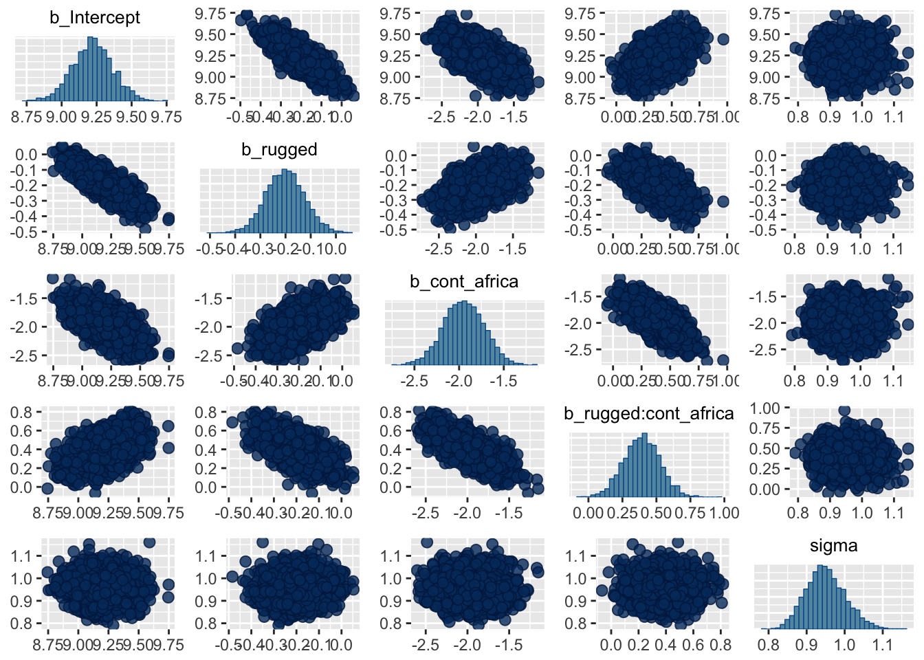

library(GGally)
post %>%
    select(b_Intercept:sigma) %>%
    ggpairs() +
    labs(subtitle = "Coefficients plot") +
    theme_ipsum()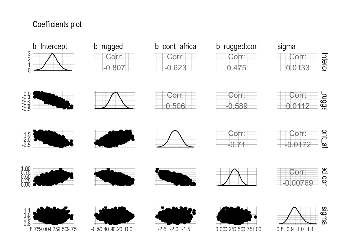

8.3.5. Using the samples

summary(m8.1, loo = T, waic = T)

##  Family: gaussian 
##   Links: mu = identity; sigma = identity 
## Formula: log_gdp ~ 1 + rugged + cont_africa + rugged:cont_africa 
##    Data: dd.trim (Number of observations: 170) 
## Samples: 4 chains, each with iter = 2000; warmup = 1000; thin = 1; 
##          total post-warmup samples = 4000
##     ICs: LOO = 469.14; WAIC = 469.02; R2 = NA
##  
## Population-Level Effects: 
##                    Estimate Est.Error l-95% CI u-95% CI Eff.Sample Rhat
## Intercept              9.22      0.14     8.94     9.51       2943 1.00
## rugged                -0.20      0.08    -0.35    -0.05       2753 1.00
## cont_africa           -1.95      0.23    -2.39    -1.51       2631 1.00
## rugged:cont_africa     0.39      0.13     0.13     0.65       2392 1.00
## 
## Family Specific Parameters: 
##       Estimate Est.Error l-95% CI u-95% CI Eff.Sample Rhat
## sigma     0.95      0.05     0.86     1.06       4000 1.00
## 
## Samples were drawn using sampling(NUTS). For each parameter, Eff.Sample 
## is a crude measure of effective sample size, and Rhat is the potential 
## scale reduction factor on split chains (at convergence, Rhat = 1).

The information criteria haven’t taken long to estimate in the models discussed so far. As your models become more complex and as your data get larger, the time their information criteria will take to compute will increase. So, if you have a complex multilevel model with a large data set, you might be better off computing the information criteria separately from the model summary.

8.3.6. Checking the chain

Visual MCMC diagnostics using the bayesplot package.

The most broadly useful tool for diagnosing malfunction is a trace plot. A trace plot merely plots the samples in sequential order, joined by a line.

We look for two things in trace plots: stationarity and good mixing.

Stationarity refers to the path staying within the posterior distribution. Notice that these traces, for example, all stick around a very stable central tendency, the center of gravity of each dimension of the posterior. Another way to think of this is that the mean value of the chain is quite stable from beginning to end.

plot(m8.1)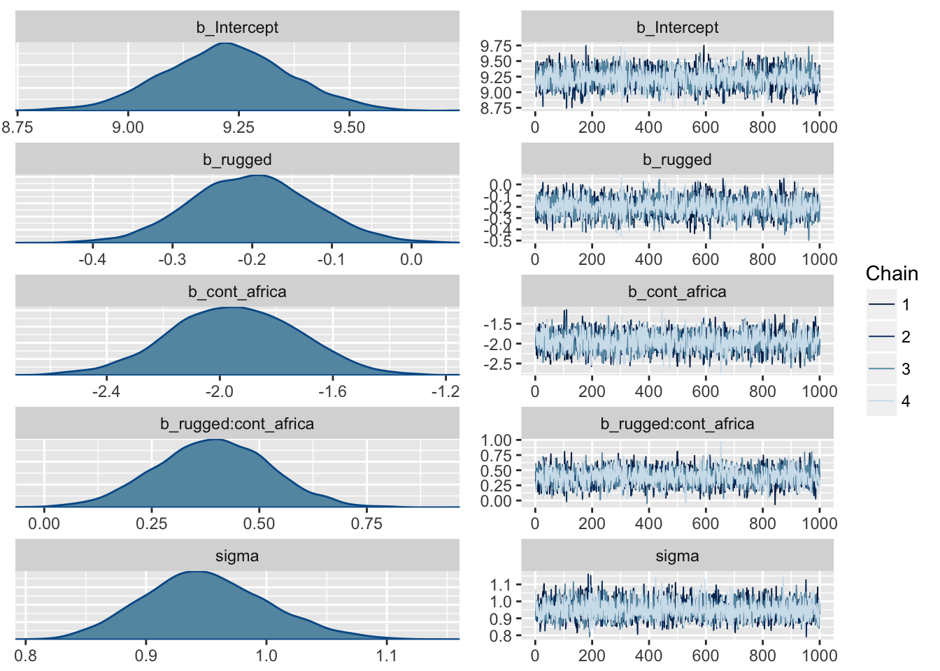

For further control, use the bayesplot package.

library(bayesplot)

post <- posterior_samples(m8.1, add_chain = T)

mcmc_trace(post[, c(1:5, 7)], # We need to include column 7 because that contains the chain info 
           facet_args = list(ncol = 3), 
           size = .15) +
    labs(title = "My custom trace plots") +
    scale_color_ipsum() +
    theme_ipsum() +
    theme(legend.position = c(.95, .2))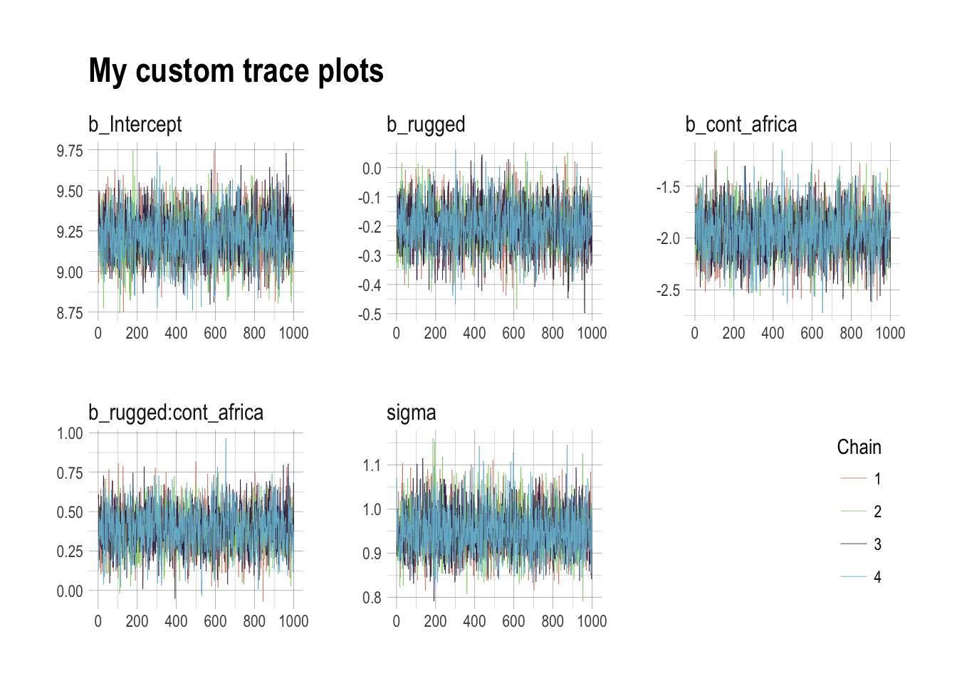

A well-mixing chain means that each successive sample within each parameter is not highly correlated with the sample before it (autocorrelation plots are good for this). Visually, you can see this by the rapid zig-zag motion of each path, as the trace traverses the posterior distribution without getting mired anyplace.

mcmc_acf(post, 
         pars = c("b_Intercept", "b_rugged", "b_cont_africa", "b_rugged:cont_africa", "sigma"),
         lags = 5) +
    scale_color_ipsum() +
    theme_ipsum()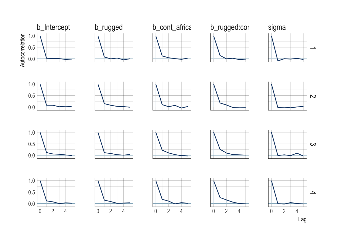

Raw Stan model code

stancode(m8.1)

## // generated with brms 2.1.0
## functions { 
## } 
## data { 
##   int<lower=1> N;  // total number of observations 
##   vector[N] Y;  // response variable 
##   int<lower=1> K;  // number of population-level effects 
##   matrix[N, K] X;  // population-level design matrix 
##   int prior_only;  // should the likelihood be ignored? 
## } 
## transformed data { 
##   int Kc = K - 1; 
##   matrix[N, K - 1] Xc;  // centered version of X 
##   vector[K - 1] means_X;  // column means of X before centering 
##   for (i in 2:K) { 
##     means_X[i - 1] = mean(X[, i]); 
##     Xc[, i - 1] = X[, i] - means_X[i - 1]; 
##   } 
## } 
## parameters { 
##   vector[Kc] b;  // population-level effects 
##   real temp_Intercept;  // temporary intercept 
##   real<lower=0> sigma;  // residual SD 
## } 
## transformed parameters { 
## } 
## model { 
##   vector[N] mu = Xc * b + temp_Intercept; 
##   // priors including all constants 
##   target += normal_lpdf(b | 0,10); 
##   target += normal_lpdf(temp_Intercept | 0,100); 
##   target += cauchy_lpdf(sigma | 0,2)
##     - 1 * cauchy_lccdf(0 | 0,2); 
##   // likelihood including all constants 
##   if (!prior_only) { 
##     target += normal_lpdf(Y | mu, sigma); 
##   } 
## } 
## generated quantities { 
##   // actual population-level intercept 
##   real b_Intercept = temp_Intercept - dot_product(means_X, b); 
## }

8.4. Care and feeding of your Markov chain

8.4.1. How many samples do you need?

It depends. First, what really matters is the effective number of samples, not the raw number. The effective number of samples is an estimate of the number of independent samples from the posterior distribution. Markov chains are typically autocorrelated, so that sequential samples are not entirely independent. Stan chains tend to be less autocorrelated than those produced by other engines, but there is always some autocorrelation. Stan provides an estimate of effective number of samples as n_eff.

Second, what do you want to know? If all you want are posterior means, it doesn’t take many samples at all to get very good estimates. Even a couple hundred samples will do. But if you care about the exact shape in the extreme tails of the posterior, the 99th percentile or so, then you’ll need many many more.

There is no universally useful number of samples to aim for. In most typical regression applications, you can get a very good estimate of the posterior mean with as few as 200 effective samples. And if the posterior is approximately Gaussian, then all you need in addition is a good estimate of the variance, which can be had with one order of magnitude more, in most cases. For highly skewed posteriors, you’ll have to think more about which region of the distribution interests you.

The warmup setting is more subtle. On the one hand, you want to have the shortest warmup period necessary, so you can get on with real sampling. But on the other hand, more warmup can mean more efficient sampling. With Stan models, typically you can devote as much as half of your total samples, the iter value, to warmup and come out very well. But for simple models like those you’ve fit so far, much less warmup is really needed. Models can vary a lot in the shape of their posterior distributions, so again there is no universally best answer.

Warmup is not burn-in. Other MCMC algorithms and software often discuss burn-in. It is conventional and useful to trim off the front of the chain, the “burn-in” phase. This is done because it is unlikely that the chain has reached stationarity within the first few samples. But Stan’s sampling algorithms use a different approach. What Stan does during warmup is quite different from what it does after warmup. The warmup samples are used to adapt sampling, and so are not actually part of the target posterior distribution at all, no matter how long warmup continues. When real sampling begins, the samples will be immediately from the target distribution, assuming adaptation was successful.

8.4.2. How many chains do you need?

How many chains do we need? There are three answers to this question. First, when debugging a model, use a single chain. Then when deciding whether the chains are valid, you need more than one chain. Third, when you begin the final run that you’ll make inferences from, you only really need one chain. But using more than one chain is fine, as well. It just doesn’t matter, once you’re sure it’s working.

For typical regression models, you can live by the motto four short chains to check, one long chain for inference.

8.4.3. Taming a wild chain

m8.2 <-
    brm(data = list(y = c(-1, 1)), 
        family = gaussian,
        y ~ 1,
        prior = c(set_prior("uniform(-1e10, 1e10)", class = "Intercept"),
                  set_prior("uniform(0, 1e10)", class = "sigma")),
        inits = list(list(Intercept = 0, sigma = 1),
                     list(Intercept = 0, sigma = 1)),
        chains = 2, iter = 4000, warmup = 1000)

## Warning: It appears as if you have specified an upper bounded prior on a parameter that has no natural upper bound.
## If this is really what you want, please specify argument 'ub' of 'set_prior' appropriately.
## Warning occurred for prior 
## sigma ~ uniform(0, 1e10)

## 
## SAMPLING FOR MODEL 'gaussian brms-model' NOW (CHAIN 1).
## 
## Gradient evaluation took 1.4e-05 seconds
## 1000 transitions using 10 leapfrog steps per transition would take 0.14 seconds.
## Adjust your expectations accordingly!
## 
## 
## Iteration:    1 / 4000 [  0%]  (Warmup)
## Iteration:  400 / 4000 [ 10%]  (Warmup)
## Iteration:  800 / 4000 [ 20%]  (Warmup)
## Iteration: 1001 / 4000 [ 25%]  (Sampling)
## Iteration: 1400 / 4000 [ 35%]  (Sampling)
## Iteration: 1800 / 4000 [ 45%]  (Sampling)
## Iteration: 2200 / 4000 [ 55%]  (Sampling)
## Iteration: 2600 / 4000 [ 65%]  (Sampling)
## Iteration: 3000 / 4000 [ 75%]  (Sampling)
## Iteration: 3400 / 4000 [ 85%]  (Sampling)
## Iteration: 3800 / 4000 [ 95%]  (Sampling)
## Iteration: 4000 / 4000 [100%]  (Sampling)
## 
##  Elapsed Time: 0.15104 seconds (Warm-up)
##                0.904563 seconds (Sampling)
##                1.0556 seconds (Total)
## 
## 
## SAMPLING FOR MODEL 'gaussian brms-model' NOW (CHAIN 2).
## 
## Gradient evaluation took 4e-06 seconds
## 1000 transitions using 10 leapfrog steps per transition would take 0.04 seconds.
## Adjust your expectations accordingly!
## 
## 
## Iteration:    1 / 4000 [  0%]  (Warmup)
## Iteration:  400 / 4000 [ 10%]  (Warmup)
## Iteration:  800 / 4000 [ 20%]  (Warmup)
## Iteration: 1001 / 4000 [ 25%]  (Sampling)
## Iteration: 1400 / 4000 [ 35%]  (Sampling)
## Iteration: 1800 / 4000 [ 45%]  (Sampling)
## Iteration: 2200 / 4000 [ 55%]  (Sampling)
## Iteration: 2600 / 4000 [ 65%]  (Sampling)
## Iteration: 3000 / 4000 [ 75%]  (Sampling)
## Iteration: 3400 / 4000 [ 85%]  (Sampling)
## Iteration: 3800 / 4000 [ 95%]  (Sampling)
## Iteration: 4000 / 4000 [100%]  (Sampling)
## 
##  Elapsed Time: 0.193866 seconds (Warm-up)
##                1.86349 seconds (Sampling)
##                2.05736 seconds (Total)

## Warning: There were 411 divergent transitions after warmup. Increasing adapt_delta above 0.8 may help. See
## http://mc-stan.org/misc/warnings.html#divergent-transitions-after-warmup

## Warning: There were 452 transitions after warmup that exceeded the maximum treedepth. Increase max_treedepth above 10. See
## http://mc-stan.org/misc/warnings.html#maximum-treedepth-exceeded

## Warning: There were 2 chains where the estimated Bayesian Fraction of Missing Information was low. See
## http://mc-stan.org/misc/warnings.html#bfmi-low

## Warning: Examine the pairs() plot to diagnose sampling problems

print(m8.2)

## Warning: There were 411 divergent transitions after warmup. Increasing adapt_delta above 0.8 may help.
## See http://mc-stan.org/misc/warnings.html#divergent-transitions-after-warmup

##  Family: gaussian 
##   Links: mu = identity; sigma = identity 
## Formula: y ~ 1 
##    Data: list(y = c(-1, 1)) (Number of observations: 2) 
## Samples: 2 chains, each with iter = 4000; warmup = 1000; thin = 1; 
##          total post-warmup samples = 6000
##     ICs: LOO = NA; WAIC = NA; R2 = NA
##  
## Population-Level Effects: 
##              Estimate    Est.Error      l-95% CI     u-95% CI Eff.Sample
## Intercept -9381278.35 264223729.30 -747487598.08 536966887.33         47
##           Rhat
## Intercept 1.03
## 
## Family Specific Parameters: 
##           Estimate     Est.Error l-95% CI      u-95% CI Eff.Sample Rhat
## sigma 348895812.70 1049117124.27 75477.37 3613144907.13         47 1.04
## 
## Samples were drawn using sampling(NUTS). For each parameter, Eff.Sample 
## is a crude measure of effective sample size, and Rhat is the potential 
## scale reduction factor on split chains (at convergence, Rhat = 1).

An Rhat value of 1.01 is suspicious. An Rhat of 1.10 indicates a catastrophe.

post <- posterior_samples(m8.2, add_chain = T)

mcmc_trace(post[, c(1:2, 4)],
           size = .25) +
    labs(title = "Sick Markov chain",
         subtitle = "These trace plots do not look like the fuzzy caterpillars we usually hope for.") +
    scale_color_ipsum() +
    theme_ipsum() +
    theme(legend.position = c(.85, 1.5),
          legend.direction = "horizontal")

## Scale for 'colour' is already present. Adding another scale for
## 'colour', which will replace the existing scale.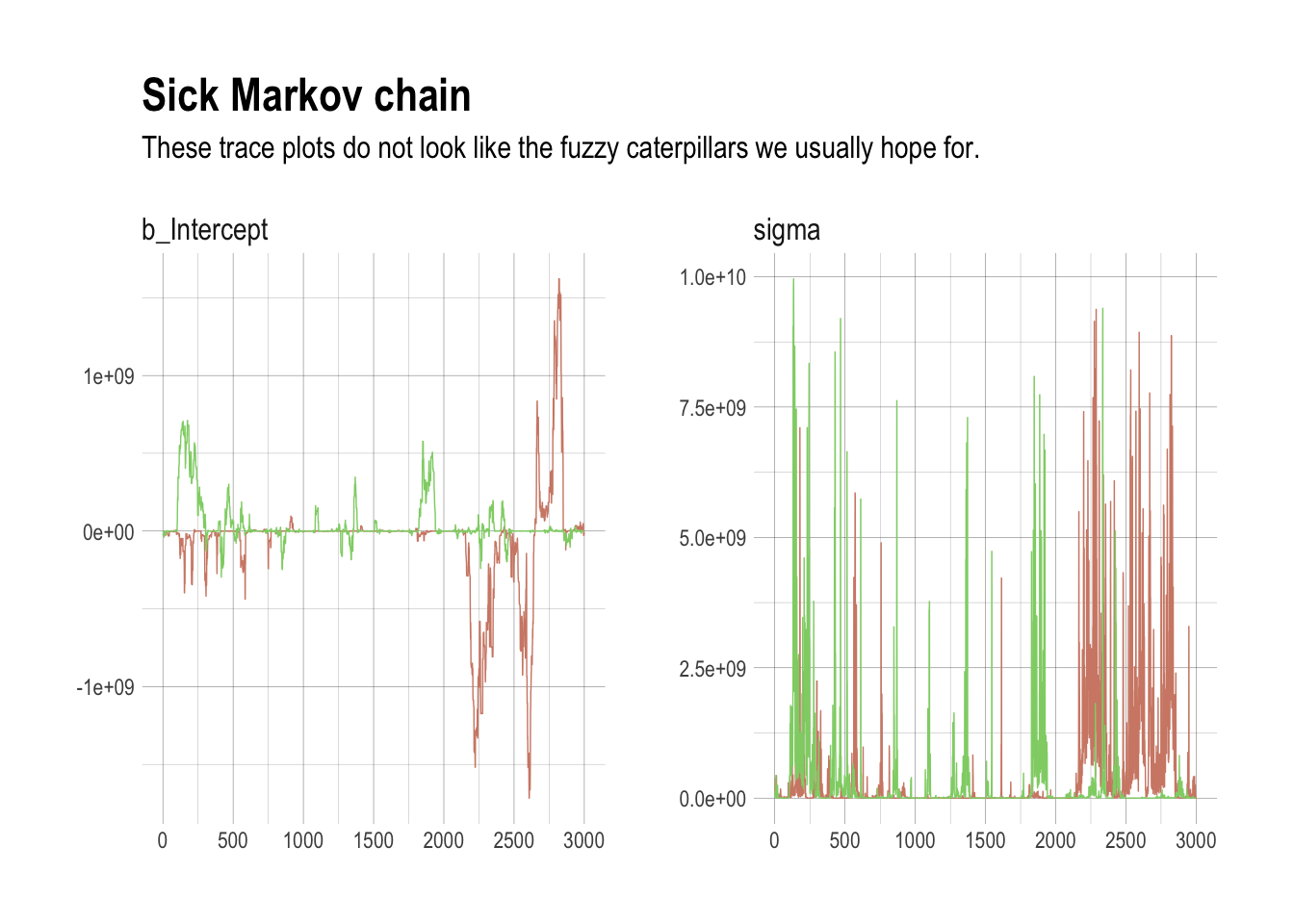

The reason the model above drifts wildly in both dimensions is that there is very little data, just two observations, and flat priors. The flat priors say that every possible value of the parameter is equally plausible, a priori. It’s easy to tame this particular chain by using weakly informative priors.

m8.3 <- brm(data = list(y = c(-1, 1)),
            y ~ 1,
            prior = c(set_prior("normal(1,10)", class = "Intercept"),
                      set_prior("cauchy(0,1)", class = "sigma")),
            inits = list(list(Intercept = 0, sigma = 1),
                         list(Intercept = 0, sigma = 1)),
            chains = 2, iter = 4000, warmup = 1000)

## 
## SAMPLING FOR MODEL 'gaussian brms-model' NOW (CHAIN 1).
## 
## Gradient evaluation took 1.3e-05 seconds
## 1000 transitions using 10 leapfrog steps per transition would take 0.13 seconds.
## Adjust your expectations accordingly!
## 
## 
## Iteration:    1 / 4000 [  0%]  (Warmup)
## Iteration:  400 / 4000 [ 10%]  (Warmup)
## Iteration:  800 / 4000 [ 20%]  (Warmup)
## Iteration: 1001 / 4000 [ 25%]  (Sampling)
## Iteration: 1400 / 4000 [ 35%]  (Sampling)
## Iteration: 1800 / 4000 [ 45%]  (Sampling)
## Iteration: 2200 / 4000 [ 55%]  (Sampling)
## Iteration: 2600 / 4000 [ 65%]  (Sampling)
## Iteration: 3000 / 4000 [ 75%]  (Sampling)
## Iteration: 3400 / 4000 [ 85%]  (Sampling)
## Iteration: 3800 / 4000 [ 95%]  (Sampling)
## Iteration: 4000 / 4000 [100%]  (Sampling)
## 
##  Elapsed Time: 0.021936 seconds (Warm-up)
##                0.054249 seconds (Sampling)
##                0.076185 seconds (Total)
## 
## 
## SAMPLING FOR MODEL 'gaussian brms-model' NOW (CHAIN 2).
## 
## Gradient evaluation took 5e-06 seconds
## 1000 transitions using 10 leapfrog steps per transition would take 0.05 seconds.
## Adjust your expectations accordingly!
## 
## 
## Iteration:    1 / 4000 [  0%]  (Warmup)
## Iteration:  400 / 4000 [ 10%]  (Warmup)
## Iteration:  800 / 4000 [ 20%]  (Warmup)
## Iteration: 1001 / 4000 [ 25%]  (Sampling)
## Iteration: 1400 / 4000 [ 35%]  (Sampling)
## Iteration: 1800 / 4000 [ 45%]  (Sampling)
## Iteration: 2200 / 4000 [ 55%]  (Sampling)
## Iteration: 2600 / 4000 [ 65%]  (Sampling)
## Iteration: 3000 / 4000 [ 75%]  (Sampling)
## Iteration: 3400 / 4000 [ 85%]  (Sampling)
## Iteration: 3800 / 4000 [ 95%]  (Sampling)
## Iteration: 4000 / 4000 [100%]  (Sampling)
## 
##  Elapsed Time: 0.020247 seconds (Warm-up)
##                0.058205 seconds (Sampling)
##                0.078452 seconds (Total)

print(m8.3)

##  Family: gaussian 
##   Links: mu = identity; sigma = identity 
## Formula: y ~ 1 
##    Data: list(y = c(-1, 1)) (Number of observations: 2) 
## Samples: 2 chains, each with iter = 4000; warmup = 1000; thin = 1; 
##          total post-warmup samples = 6000
##     ICs: LOO = NA; WAIC = NA; R2 = NA
##  
## Population-Level Effects: 
##           Estimate Est.Error l-95% CI u-95% CI Eff.Sample Rhat
## Intercept    -0.02      1.70    -3.63     3.32        751 1.00
## 
## Family Specific Parameters: 
##       Estimate Est.Error l-95% CI u-95% CI Eff.Sample Rhat
## sigma     2.04      1.82     0.63     6.64        848 1.00
## 
## Samples were drawn using sampling(NUTS). For each parameter, Eff.Sample 
## is a crude measure of effective sample size, and Rhat is the potential 
## scale reduction factor on split chains (at convergence, Rhat = 1).

post <- posterior_samples(m8.3, add_chain = T)

mcmc_trace(post[, c(1:2, 4)],
           size = .25) +
    labs(title = "Healthy Markov chain",
         subtitle = "Oh man. This looks so much better.") +
    scale_color_ipsum() +
    theme_ipsum() +
    theme(legend.position = c(.85, 1.5),
          legend.direction = "horizontal")

## Scale for 'colour' is already present. Adding another scale for
## 'colour', which will replace the existing scale.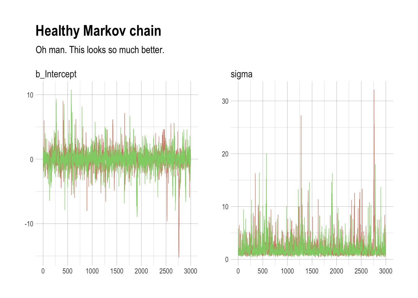

library(gridExtra)

## 
## Attaching package: 'gridExtra'

## The following object is masked from 'package:dplyr':
## 
##     combine

intercept <- post %>%
    select(b_Intercept) %>%
    ggplot(aes(x = b_Intercept)) +
    stat_density(geom = "line") +
    geom_line(data = data.frame(x = seq(from = min(post$b_Intercept),
                                        to = max(post$b_Intercept),
                                        length.out = 50)),
              aes(x = x, y = dnorm(x = x, mean = 1, sd = 10)),
              color = ipsum_pal()(1), linetype = 2) +
    theme_ipsum()

sigma <-  post %>%
    select(sigma) %>%
    ggplot(aes(x = sigma)) +
    stat_density(geom = "line") +
    geom_line(data = data.frame(x = seq(from = 0,
                                        to = max(post$sigma),
                                        length.out = 50)),
              aes(x = x, y = dcauchy(x = x, location = 0, scale = 1)*2),
              color = ipsum_pal()(2)[2], linetype = 2) +
    coord_cartesian(xlim = c(0, 10)) +
    theme_ipsum()

grid.arrange(intercept, sigma, ncol=2)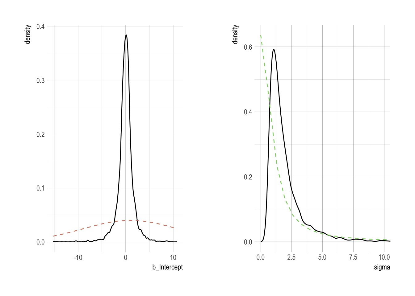

8.4.4. Non-identifiable parameters

set.seed(8.4)
y <- rnorm(100, mean = 0, sd = 1)

m8.4 <-
    brm(data = list(y = y,
                    intercept1 = 1,
                    intercept2 = 1), 
        family = gaussian,
        y ~ 0 + intercept1 + intercept2,
        prior = c(set_prior("uniform(-1e10, 1e10)", class = "b"),
                  set_prior("cauchy(0, 1)", class = "sigma")),
        inits = list(list(intercept1 = 0, intercept2 = 0, sigma = 1),
                     list(intercept1 = 0, intercept2 = 0, sigma = 1)),
        chains = 2, iter = 4000, warmup = 1000,
        seed = 8.4)

## Warning: It appears as if you have specified a lower bounded prior on a parameter that has no natural lower bound.
## If this is really what you want, please specify argument 'lb' of 'set_prior' appropriately.
## Warning occurred for prior 
## b ~ uniform(-1e10, 1e10)

## Warning: It appears as if you have specified an upper bounded prior on a parameter that has no natural upper bound.
## If this is really what you want, please specify argument 'ub' of 'set_prior' appropriately.
## Warning occurred for prior 
## b ~ uniform(-1e10, 1e10)

## 
## SAMPLING FOR MODEL 'gaussian brms-model' NOW (CHAIN 1).
## 
## Gradient evaluation took 3.6e-05 seconds
## 1000 transitions using 10 leapfrog steps per transition would take 0.36 seconds.
## Adjust your expectations accordingly!
## 
## 
## Iteration:    1 / 4000 [  0%]  (Warmup)
## Iteration:  400 / 4000 [ 10%]  (Warmup)
## Iteration:  800 / 4000 [ 20%]  (Warmup)
## Iteration: 1001 / 4000 [ 25%]  (Sampling)
## Iteration: 1400 / 4000 [ 35%]  (Sampling)
## Iteration: 1800 / 4000 [ 45%]  (Sampling)
## Iteration: 2200 / 4000 [ 55%]  (Sampling)
## Iteration: 2600 / 4000 [ 65%]  (Sampling)
## Iteration: 3000 / 4000 [ 75%]  (Sampling)
## Iteration: 3400 / 4000 [ 85%]  (Sampling)
## Iteration: 3800 / 4000 [ 95%]  (Sampling)
## Iteration: 4000 / 4000 [100%]  (Sampling)
## 
##  Elapsed Time: 4.25438 seconds (Warm-up)
##                14.7496 seconds (Sampling)
##                19.004 seconds (Total)
## 
## 
## SAMPLING FOR MODEL 'gaussian brms-model' NOW (CHAIN 2).
## 
## Gradient evaluation took 1.2e-05 seconds
## 1000 transitions using 10 leapfrog steps per transition would take 0.12 seconds.
## Adjust your expectations accordingly!
## 
## 
## Iteration:    1 / 4000 [  0%]  (Warmup)
## Iteration:  400 / 4000 [ 10%]  (Warmup)
## Iteration:  800 / 4000 [ 20%]  (Warmup)
## Iteration: 1001 / 4000 [ 25%]  (Sampling)
## Iteration: 1400 / 4000 [ 35%]  (Sampling)
## Iteration: 1800 / 4000 [ 45%]  (Sampling)
## Iteration: 2200 / 4000 [ 55%]  (Sampling)
## Iteration: 2600 / 4000 [ 65%]  (Sampling)
## Iteration: 3000 / 4000 [ 75%]  (Sampling)
## Iteration: 3400 / 4000 [ 85%]  (Sampling)
## Iteration: 3800 / 4000 [ 95%]  (Sampling)
## Iteration: 4000 / 4000 [100%]  (Sampling)
## 
##  Elapsed Time: 4.18079 seconds (Warm-up)
##                14.8124 seconds (Sampling)
##                18.9931 seconds (Total)

## Warning: There were 4922 transitions after warmup that exceeded the maximum treedepth. Increase max_treedepth above 10. See
## http://mc-stan.org/misc/warnings.html#maximum-treedepth-exceeded

## Warning: Examine the pairs() plot to diagnose sampling problems

print(m8.4)

## Warning: The model has not converged (some Rhats are > 1.1). Do not analyse the results! 
## We recommend running more iterations and/or setting stronger priors.

##  Family: gaussian 
##   Links: mu = identity; sigma = identity 
## Formula: y ~ 0 + intercept1 + intercept2 
##    Data: list(y = y, intercept1 = 1, intercept2 = 1) (Number of observations: 100) 
## Samples: 2 chains, each with iter = 4000; warmup = 1000; thin = 1; 
##          total post-warmup samples = 6000
##     ICs: LOO = NA; WAIC = NA; R2 = NA
##  
## Population-Level Effects: 
##            Estimate Est.Error l-95% CI u-95% CI Eff.Sample Rhat
## intercept1  1116.48    944.73  -762.62  2439.62          2 2.50
## intercept2 -1116.57    944.74 -2439.65   762.38          2 2.50
## 
## Family Specific Parameters: 
##       Estimate Est.Error l-95% CI u-95% CI Eff.Sample Rhat
## sigma     1.06      0.08     0.91     1.22          5 1.16
## 
## Samples were drawn using sampling(NUTS). For each parameter, Eff.Sample 
## is a crude measure of effective sample size, and Rhat is the potential 
## scale reduction factor on split chains (at convergence, Rhat = 1).

post <- posterior_samples(m8.4, add_chain = T)

mcmc_trace(post[, c(1:3, 5)],
           size = .25) +
    labs(title = "Trace Plot") +
    scale_color_ipsum() +
    theme_ipsum() +
    theme(legend.position = c(.85, 1.5),
          legend.direction = "horizontal")

## Scale for 'colour' is already present. Adding another scale for
## 'colour', which will replace the existing scale.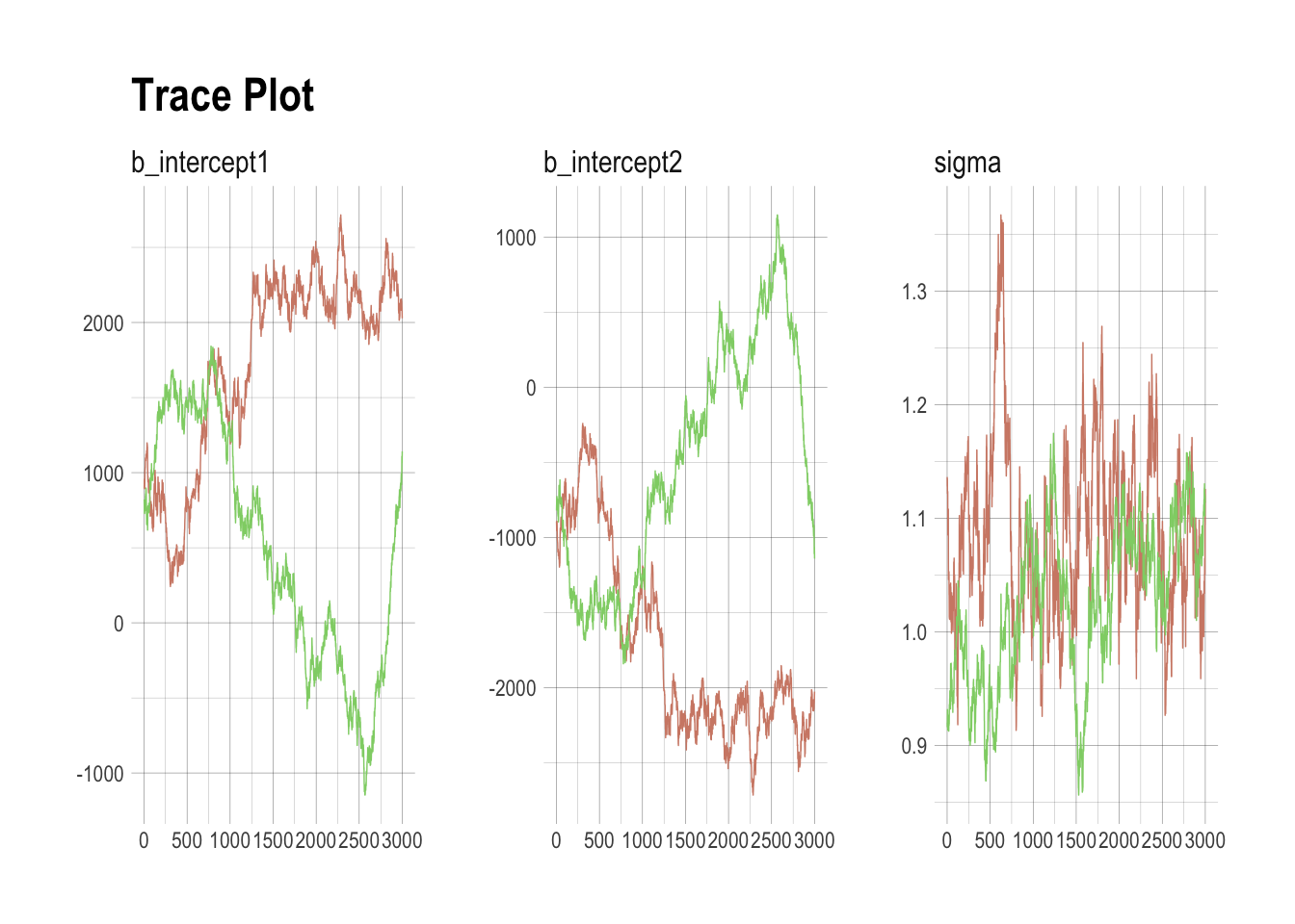

m8.5 <-
    brm(data = list(y = y,
                    intercept1 = 1,
                    intercept2 = 1), 
        family = gaussian,
        y ~ 0 + intercept1 + intercept2,
        prior = c(set_prior("normal(0, 10)", class = "b"),
                  set_prior("cauchy(0, 1)", class = "sigma")),
        inits = list(list(intercept1 = 0, intercept2 = 0, sigma = 1),
                     list(intercept1 = 0, intercept2 = 0, sigma = 1)),
        chains = 2, iter = 4000, warmup = 1000)

## 
## SAMPLING FOR MODEL 'gaussian brms-model' NOW (CHAIN 1).
## 
## Gradient evaluation took 3.6e-05 seconds
## 1000 transitions using 10 leapfrog steps per transition would take 0.36 seconds.
## Adjust your expectations accordingly!
## 
## 
## Iteration:    1 / 4000 [  0%]  (Warmup)
## Iteration:  400 / 4000 [ 10%]  (Warmup)
## Iteration:  800 / 4000 [ 20%]  (Warmup)
## Iteration: 1001 / 4000 [ 25%]  (Sampling)
## Iteration: 1400 / 4000 [ 35%]  (Sampling)
## Iteration: 1800 / 4000 [ 45%]  (Sampling)
## Iteration: 2200 / 4000 [ 55%]  (Sampling)
## Iteration: 2600 / 4000 [ 65%]  (Sampling)
## Iteration: 3000 / 4000 [ 75%]  (Sampling)
## Iteration: 3400 / 4000 [ 85%]  (Sampling)
## Iteration: 3800 / 4000 [ 95%]  (Sampling)
## Iteration: 4000 / 4000 [100%]  (Sampling)
## 
##  Elapsed Time: 1.01711 seconds (Warm-up)
##                3.38167 seconds (Sampling)
##                4.39879 seconds (Total)
## 
## 
## SAMPLING FOR MODEL 'gaussian brms-model' NOW (CHAIN 2).
## 
## Gradient evaluation took 1.6e-05 seconds
## 1000 transitions using 10 leapfrog steps per transition would take 0.16 seconds.
## Adjust your expectations accordingly!
## 
## 
## Iteration:    1 / 4000 [  0%]  (Warmup)
## Iteration:  400 / 4000 [ 10%]  (Warmup)
## Iteration:  800 / 4000 [ 20%]  (Warmup)
## Iteration: 1001 / 4000 [ 25%]  (Sampling)
## Iteration: 1400 / 4000 [ 35%]  (Sampling)
## Iteration: 1800 / 4000 [ 45%]  (Sampling)
## Iteration: 2200 / 4000 [ 55%]  (Sampling)
## Iteration: 2600 / 4000 [ 65%]  (Sampling)
## Iteration: 3000 / 4000 [ 75%]  (Sampling)
## Iteration: 3400 / 4000 [ 85%]  (Sampling)
## Iteration: 3800 / 4000 [ 95%]  (Sampling)
## Iteration: 4000 / 4000 [100%]  (Sampling)
## 
##  Elapsed Time: 0.978612 seconds (Warm-up)
##                3.85508 seconds (Sampling)
##                4.83369 seconds (Total)

print(m8.5)

##  Family: gaussian 
##   Links: mu = identity; sigma = identity 
## Formula: y ~ 0 + intercept1 + intercept2 
##    Data: list(y = y, intercept1 = 1, intercept2 = 1) (Number of observations: 100) 
## Samples: 2 chains, each with iter = 4000; warmup = 1000; thin = 1; 
##          total post-warmup samples = 6000
##     ICs: LOO = NA; WAIC = NA; R2 = NA
##  
## Population-Level Effects: 
##            Estimate Est.Error l-95% CI u-95% CI Eff.Sample Rhat
## intercept1     0.20      7.11   -14.03    14.12       1192 1.00
## intercept2    -0.29      7.11   -14.22    13.96       1191 1.00
## 
## Family Specific Parameters: 
##       Estimate Est.Error l-95% CI u-95% CI Eff.Sample Rhat
## sigma     1.09      0.08     0.95     1.25       2116 1.00
## 
## Samples were drawn using sampling(NUTS). For each parameter, Eff.Sample 
## is a crude measure of effective sample size, and Rhat is the potential 
## scale reduction factor on split chains (at convergence, Rhat = 1).

post <- posterior_samples(m8.5, add_chain = T)

mcmc_trace(post[, c(1:3, 5)],
           size = .25) +
    labs(title = "Trace Plot") +
    scale_color_ipsum() +
    theme_ipsum() +
    theme(legend.position = c(.85, 1.5),
          legend.direction = "horizontal")

## Scale for 'colour' is already present. Adding another scale for
## 'colour', which will replace the existing scale.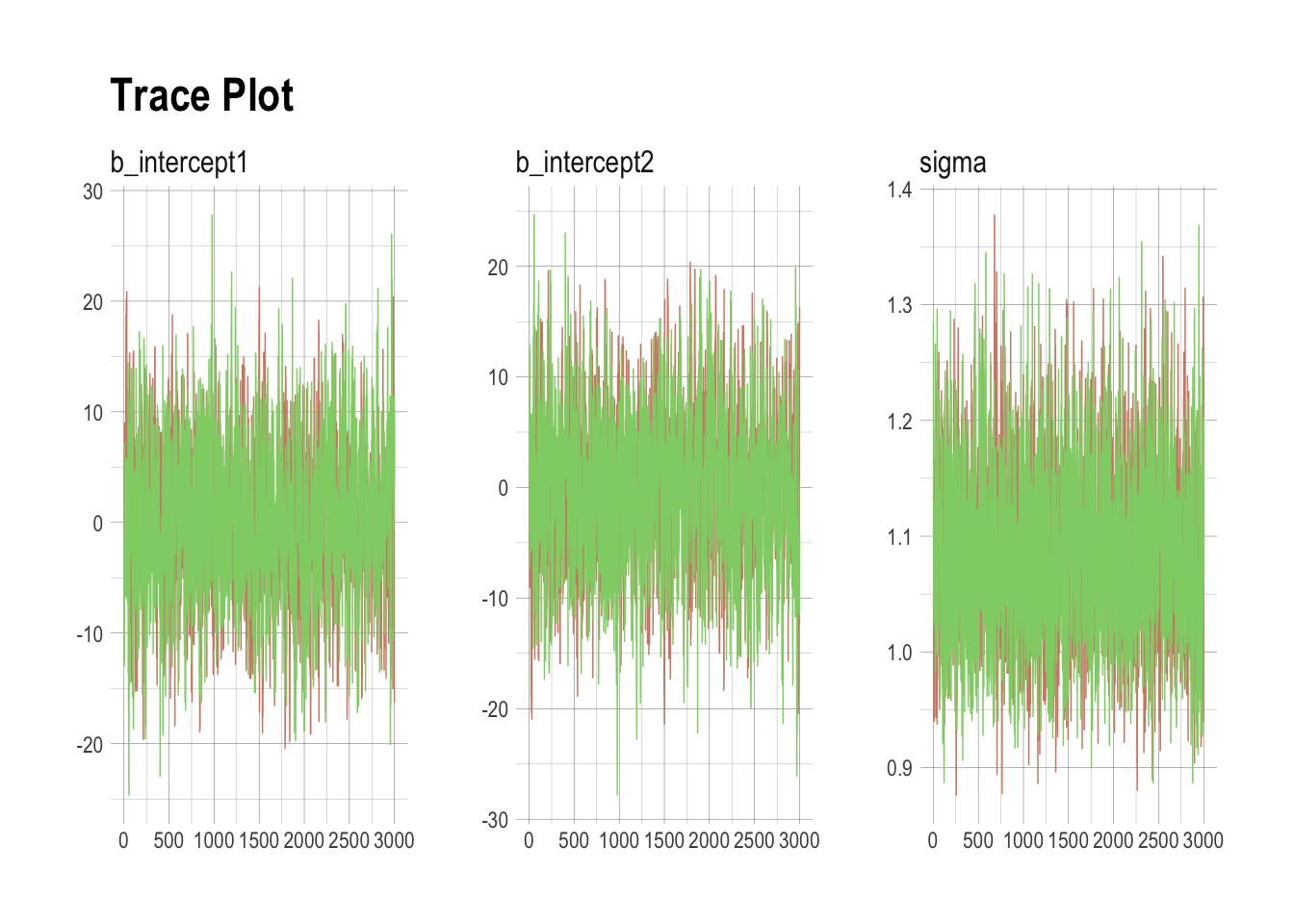

Folk theorem of statistical computing: When you are having trouble fitting a model, it often indicates a bad model. Often, a model that is very slow to sample is under-identified.

Check prior choice recommendations.

References

McElreath, R. (2016). Statistical rethinking: A Bayesian course with examples in R and Stan. Chapman & Hall/CRC Press.

Kurz, A. S. (2018, March 9). brms, ggplot2 and tidyverse code, by chapter. Retrieved from https://goo.gl/JbvNTj

bayesian notes