Entropy provides one useful principle to guide choice of probability distributions: bet on the distribution with the biggest entropy.
First, the distribution with the biggest entropy is the widest and least informative distribution. Choosing the distribution with the largest entropy means spreading probability as evenly as possible, while still remaining consistent with anything we think we know about a process. In the context of choosing a prior, it means choosing the least informative distribution consistent with any partial scientific knowledge we have about a parameter. In the context of choosing a likelihood, it means selecting the distribution we’d get by counting up all the ways outcomes could arise, consistent with the constraints on the outcome variable. In both cases, the resulting distribution embodies the least information while remaining true to the information we’ve provided.
Second, nature tends to produce empirical distributions that have high entropy. Back in Chapter 4, I introduced the Gaussian distribution by demonstrating how any process that repeatedly adds together fluctuations will tend towards an empirical distribution with the distinctive Gaussian shape. That shape is the one that contains no information about the underlying process except its location and variance. As a result, it has maximum entropy.
Third, regardless of why it works, it tends to work. Mathematical procedures are effective even when we don’t understand them. There are no guarantees that any logic in the small world will be useful in the large world. We use logic in science because it has a strong record of effectiveness in addressing real world problems. This is the historical justification: The approach has solved difficult problems in the past. This is no guarantee that it will work on your problem. But no approach can guarantee that.
9.1. Maximum entropy
Information entropy is a measure that satisfies three criteria: (1) the measure should be continuous; (2) it should increase as the number of possible events increases; and (3) it should be additive.
\[H(p) = -\sum _{ i=1 }^{ n }p_i\ln(p_i)\]
The maximum entropy principle is: The distribution that can happen the most ways is also the distribution with the biggest information entropy. The distribution with the biggest entropy is the most conservative distribution that obeys its constraints.
# Distribution of pebbles
p <- list()
p$A <- c(0,0,10,0,0)
p$B <- c(0,1,8,1,0)
p$C <- c(0,2,6,2,0)
p$D <- c(1,2,4,2,1)
p$E <- c(2,2,2,2,2)

p_norm <- lapply( p , function(q) q/sum(q))

H <- sapply( p_norm , function(q) -sum(ifelse(q==0,0,q*log(q))) )
H
## A B C D E
## 0.0000000 0.6390319 0.9502705 1.4708085 1.6094379Information entropy is a way of counting how many unique arrangements correspond to a distribution.
The maximum entropy distribution, i.e. the most plausible distribution, is the distribution that can happen the greatest number of ways.
Therefore Bayesian inference can be seen as producing a posterior distribution that is most similar to the prior distribution as possible, while remaining logically consistent with the stated information.
9.1.1. Gaussian
A generalized normal distribution is defined by the probability density:
\[\Pr\left( { y }|{ \mu ,\alpha ,\beta } \right) =\frac { \beta }{ 2\alpha \Gamma \left( { 1 }/{ \beta } \right) } { e }^{ -{ \left( \frac { \left| y-\mu \right| }{ \alpha } \right) }^{ \beta } }\]
If all we are willing to assume about a collection of measurements is that they have a finite variance, then the Gaussian distribution represents the most conservative probability distribution to assign to those measurements.
9.1.2. Binomial
# build list of the candidate distributions
p <- list()
p[[1]] <- c(1/4,1/4,1/4,1/4)
p[[2]] <- c(2/6,1/6,1/6,2/6)
p[[3]] <- c(1/6,2/6,2/6,1/6)
p[[4]] <- c(1/8,4/8,2/8,1/8)

# compute expected value of each
sapply( p , function(p) sum(p*c(0,1,1,2)) )
## [1] 1 1 1 1# compute entropy of each distribution
sapply( p , function(p) -sum( p*log(p) ) )## [1] 1.386294 1.329661 1.329661 1.213008sim.p <- function(G=1.4) {
x123 <- runif(3)
x4 <- ( (G)*sum(x123)-x123[2]-x123[3] )/(2-G)
z <- sum( c(x123,x4) )
p <- c( x123 , x4 )/z
list( H=-sum( p*log(p) ) , p=p )
}
H <- replicate( 1e5 , sim.p(1.4) )
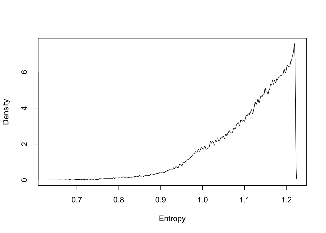
plot(density( as.numeric(H[1,]) , adj=0.1 ), main = "", xlab = "Entropy")
entropies <- as.numeric(H[1,])
distributions <- H[2,]

distributions[ which.max(entropies) ]
## [[1]]
## [1] 0.09042442 0.20930294 0.20984822 0.49042442max(entropies)## [1] 1.221726# Theoretical maximum entropy distribution
p <- 0.7
( A <- c( (1-p)^2 , p*(1-p) , (1-p)*p , p^2 ) )## [1] 0.09 0.21 0.21 0.49-sum( A*log(A) )## [1] 1.221729When only two unordered outcomes are possible and the expected numbers of each type of event are assumed to be constant, then the distribution that is most consistent with these constraints is the binomial distribution. This distribution spreads probability out as evenly and conservatively as possible. Any other distribution implies hidden constraints that are unknown to us, reflecting phantom assumptions.
If only two unordered outcomes are possible and you think the process generating them is invariant in time, so that the expected value remains constant at each combination of predictor values, then the distribution that is most conservative is the binomial.
9.2. Generalized linear models
9.2.1. Meet the family
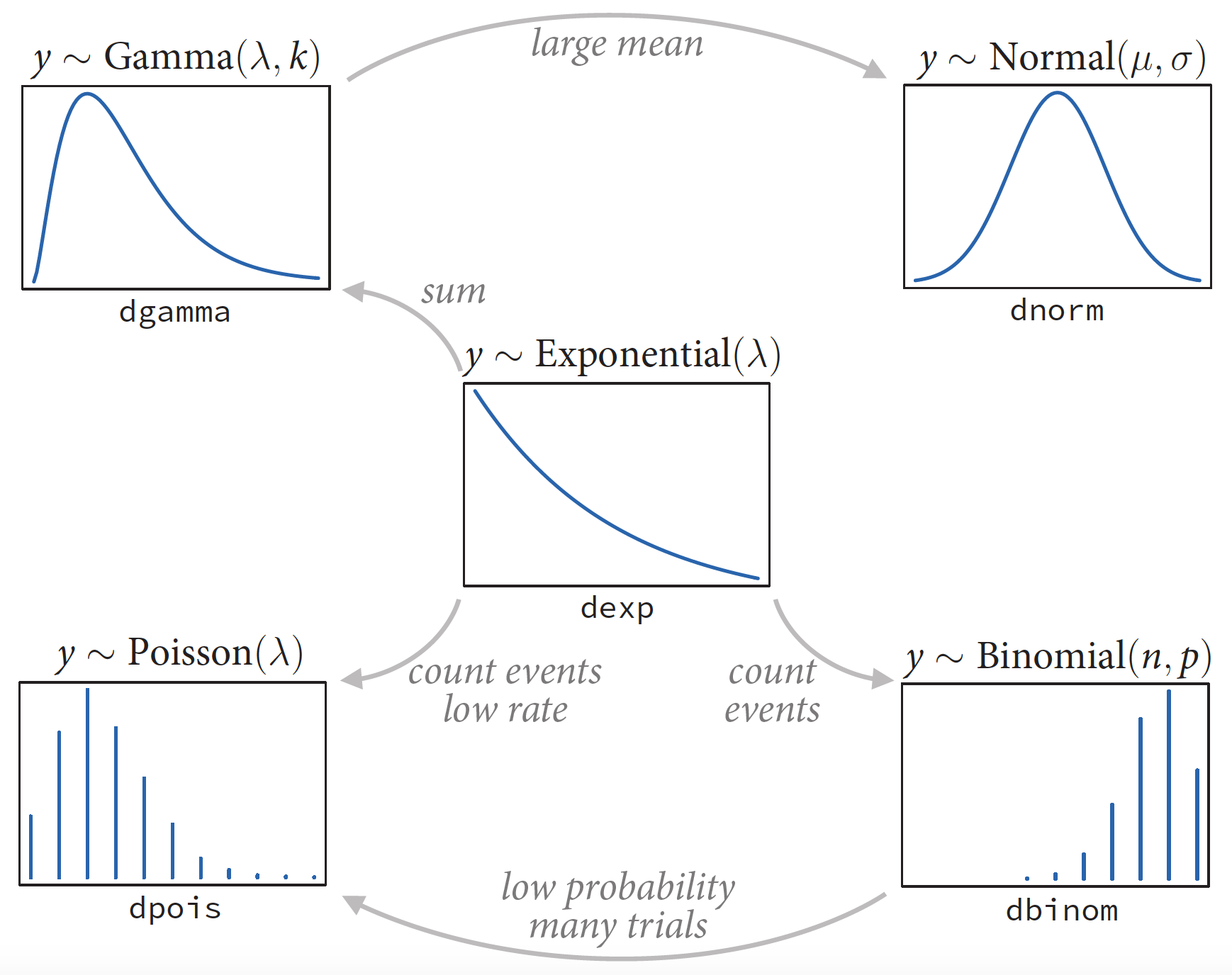
The most common distributions used in statistical modeling are members of a family known as the exponential family. Every member of this family is a maximum entropy distribution, for some set of constraints.

Exponential Family. Image from Statistical rethinking: A Bayesian course with examples in R and Stan by Richard McElreath.
The exponential distribution (center) is constrained to be zero or positive. It is a fundamental distribution of distance and duration, kinds of measurements that represent displacement from some point of reference, either in time or space. If the probability of an event is constant in time or across space, then the distribution of events tends towards exponential. The exponential distribution has maximum entropy among all non-negative continuous distributions with the same average displacement. Its shape is described by a single parameter, the rate of events \(\lambda\), or the average displacement \(\lambda^{-1}\). This distribution is the core of survival and event history analysis.
The gamma distribution (top-left) is also constrained to be zero or positive. It too is a fundamental distribution of distance and duration. But unlike the exponential distribution, the gamma distribution can have a peak above zero. If an event can only happen after two or more exponentially distributed events happen, the resulting waiting times will be gamma distributed. The gamma distribution has maximum entropy among all distributions with the same mean and same average logarithm. Its shape is described by two parameters, but there are at least three different common descriptions of these parameters, so some care is required when working with it. The gamma distribution is common in survival and event history analysis, as well as some contexts in which a continuous measurement is constrained to be positive.
The Poisson distribution (bottom-left) is a count distribution like the binomial. It is actually a special case of the binomial, mathematically. If the number of trials \(n\) is very large (and usually unknown) and the probability of a success \(p\) is very small, then a binomial distribution converges to a Poisson distribution with an expected rate of events per unit time of \(\lambda = np\). Practically, the Poisson distribution is used for counts that never get close to any theoretical maximum. As a special case of the binomial, it has maximum entropy under exactly the same constraints. Its shape is described by a single parameter, the rate of events \(\lambda\).
9.2.2. Linking linear models to distributions
A link function is required to prevent mathematical accidents like negative distances or probability masses that exceed 1. A link function’s job is to map the linear space of a model like \(\alpha + \beta x_i\) onto the non-linear space of a parameter like \(\theta\).
Logit link
The logit link maps a parameter that is defined as a probability mass, and therefore constrained to lie between zero and one, onto a linear model that can take on any real value. This link is extremely common when working with binomial GLMs.
\[\begin{eqnarray} { y }_{ i } & \sim & \text{ Binomial }(n, { p }_{ i } ) \\ \text{ logit} \left( { p }_{ i } \right) & = & \alpha +{ \beta }{ x }_{ i } \end{eqnarray}\]
where
\[\text{ logit} \left( { p }_{ i } \right) = \log \frac { { p }_{ i } }{ 1-{ p }_{ i } }\]
The “odds” of an event are just the probability it happens divided by the probability it does not happen.
Interpretation of parameter estimates changes, because no longer does a unit change in a predictor variable produce a constant change in the mean of the outcome variable.
In GLM, every predictor essentially interacts with itself, because the impact of a change in a predictor depends upon the value of the predictor before the change. More generally, every predictor variable effectively interacts with every other predictor variable, whether you explicitly model them as interactions or not. This fact makes the visualization of counter-factual predictions even more important for understanding what the model is telling you.
Log link
The log link maps a parameter that is defined over only positive real values onto a linear model.
\[\begin{eqnarray} { y }_{ i } & \sim & \text{ Normal }(\mu, { \sigma }_{ i } ) \\ \log \left( { \sigma }_{ i } \right) & = & \alpha +{ \beta }{ x }_{ i } \end{eqnarray}\]
which implies
\[\sigma_i = \exp \left( \alpha +{ \beta }{ x }_{ i } \right)\]
While using a log link does solve the problem of constraining the parameter to be positive, it may also create a problem when the model is asked to predict well outside the range of data used to fit it.
In sensitivity analysis, many justifiable analyses are tried, and all of them are described.
9.2.3. Absolute and relative differences
There is an important practical consequence of the way that a link function compresses and expands different portions of the linear model’s range: Parameter estimates do not by themselves tell you the importance of a predictor on the outcome. The reason is that each parameter represents a relative difference on the scale of the linear model, ignoring other parameters, while we are really interested in absolute differences in outcomes that must incorporate all parameters.
9.2.4. GLMs and information criteria
Only compare models that all use the same type of likelihood. Of course it is possible to compare models that use different likelihoods, just not with information criteria.
References
McElreath, R. (2016). Statistical rethinking: A Bayesian course with examples in R and Stan. Chapman & Hall/CRC Press.
Kurz, A. S. (2018, March 9). brms, ggplot2 and tidyverse code, by chapter. Retrieved from https://goo.gl/JbvNTj